Estratégia Financeira

Part 7 - Ch 14 Capital Structure in a Perfect Market

Henrique C. Martins

07-05-2024

Chapter Outline

14.1 Equity Versus Debt Financing

14.2 MM I: Leverage, Arbitrage, and Firm Value

14.3 MM II: Leverage, Risk, and the Cost of Capital

14.4 Capital Structure Fallacies

14.5 MM: Beyond the Propositions

14.1 Equity Versus Debt Financing

When corporations raise funds from outside investors, they must choose which type of security to issue.

The most common choices are financing through equity alone and financing through a combination of debt and equity.

The relative proportions of debt, equity, and other securities that a firm has outstanding constitute its capital structure.

A central question in this chapter:

If a firm decides for a specific capital structure, does it change the investment decisions?

Similarly,

Do capital structure decisions affect firm value?

For clarity: Throughout the chapter, we will assume the firm is a portfolio of debt and equity (and maybe other securities).

14.1 Equity Versus Debt Financing

Let’s start our discussion by analyzing again the value of a firm.

Imagine an economy with two future states; firm will receive cash flows as follows:

Date 0 (investment)	Date 1 (strong economy)	Date 1 (Weak economy)
-800	1400	900

The cost of capital for this project is 15%. Each scenario has a 50% probability of occurrence. The NPV is:

\[NPV = -800 + \frac{\frac{1}{2} \times 1400 + \frac{1}{2} \times 900 }{1.15} = 200\]

\[PV(CF) = \frac{1150}{1.15} = 1000\]

So the firm value today is $1000. If the firm wants to finance the project all-equity, it could raise this amount selling equity. In this case, the firm is unlevered equity.

14.1 Equity Versus Debt Financing

The expected return on the unlevered equity is 15%.

Date 0 (investment)	Date 1 (strong economy)	Date 1 (Weak economy)
1000	1400	900
Return	+40%	-10%

\[\frac{1}{2} \times 40\% + \frac{1}{2} \times -10\% = 15\%\]

14.1 Equity Versus Debt Financing

Let’s now analyse the case where the firm issues 500 of debt and 500 of equity. This firm is levered equity. The debt cost is 5%. Do the NPV and the firm value change?

Because the firm needs to pay debt holders no matter the state of the economy, we can say that Debt value in Date 1 is 525 ($500 \times 1.05$).

Because we know the firm value in each state of the economy, we can say that the difference between the firm value and the debt value is the equity value: $V - D = E$, i.e. $1400 - 525 = 875$ or $900 - 525 = 375$.

Then, we can write:

Source	Date 0 (investment)	Date 1 (strong economy)	Date 1 (Weak economy)
Debt (D)	500	525	525
Equity (E)	?	875	375
Firm (V)	1000	1400	900

14.1 Equity Versus Debt Financing

Wait, but if debt cost is only 5%, why the firm value still is 1.000? Shouldn’t the value of equity increase?

The answer is that the cost of equity increases for levered equity. Let’s see how.

Source	Date 0 (investment)	Date 1 (strong)	Date 1 (Weak)	Return 1 (strong)	Return 1 (Weak)
D	500	525	525	5%	5%
E	500	875	375	75%	-25%
V	1000	1400	900	40%	-10%

Unlevered equity has returns of 40% or -10%. On average, 15%.

Debt has return of 5% no matter what.

Levered equity has returns of 75% ($\frac{875}{500}-1$) or -25% ($\frac{375}{500}-1$). On average, 25%.

14.1 Equity Versus Debt Financing

The takeaway:

Levered equity is riskier, so the cost of capital is higher.

Source	Return sensitivity (systematic risk)	Risk premium
Debt	5% - 5% = 0%	5% - 5% = 0%
Unlevered Equity	40% - (-10%) = 50%	15% - 5% = 10%
Levered Equity	75% - (-25%) = 100%	25% - 5% = 20%

Because the debt’s return bears no systematic risk, its risk premium is zero.

In this particular case, the levered equity has twice the systematic risk of the unlevered equity and, as a result, has twice the risk premium.

Modigliani and Miller argued that with perfect capital markets, the total value of a firm should not depend on its capital structure.

They reasoned that the firm’s total cash flows still equal the cash flows of the project and, therefore, have the same present value.

14.1 Equity Versus Debt Financing

In summary

In the case of perfect capital markets, if the firm is 100% equity financed, the equity holders will require a 15% expected return.
If the firm is financed 50% with debt and 50% with equity, the debt holders will receive a return of 5%, while the levered equity holders will require an expected return of 25% (because of increased risk).
Leverage increases the risk of equity even when there is no risk that the firm will default.
- Thus, while debt may be cheaper, its use raises the cost of capital for equity. Considering both sources of capital together, the firm’s average cost of capital with leverage is the same as for the unlevered firm.

14.1 Equity Versus Debt Financing

Problem

Using the same values as before, suppose the firm borrows $700 when financing the project.

According to Modigliani and Miller, what should the value of the equity be? What is the expected return?

Because the value of the firm’s total cash flows is still 1000, if the firm borrows 700, its equity will be worth 300.

14.1 Equity Versus Debt Financing

The firm will owe 700 × 1.05 = 735 in one year to debt holders. Thus,

if the economy is strong, equity holders will receive $1400 − 735 = 665$, for a return of $\frac{665}{300}-1 = 121.67\%$.
if the economy is weak, equity holders will receive $900 − 735 = 165$, for a return of $\frac{165}{300}-1 = -45\%$.

Expected return is:

\[\frac{1}{2} \times 121.67\% + \frac{1}{2} \times -45\% = 38.33\%\]

Note that the equity has a return sensitivity of 121.67% − (−45.0%) = 166.67%.

Its risk premium is 38.33% − 5% = 33.33%.

14.1 Equity Versus Debt Financing

Source	Date 0	Date 1 (strong)	Date 1 (Weak)	Ret. 1 (strong)	Ret. 1 (Weak)	Syst. risk	Risk premium
Debt	700	735	735	5%	5%	5% - 5% = 0%	5% - 5% = 0%
Equity	300	665	165	122%	-45%	122% - (-45%) = 167%	38% - 5% = 33%
Firm	1000	1400	900	40%	-10%	75% - (-25%) = 100%	25% - 5% = 20%

So, debt increases equity risk.

14.2 MM I

In this subsection, we will explore further the MM propositions and the theory of capital structure.

First, we will understand what Homemade Leverage means.

Let’s say the firm selects a given capital structure. The investor likes an alternative capital structure.
MM demonstrated that if investors would prefer an alternative capital structure to the one the firm has chosen, investors can borrow or lend on their own and achieve the same result.

14.2 MM I

Assume the firm is an all−equity firm. An investor who would prefer to hold levered equity can do so by using leverage in his own portfolio.

An investor who would like more leverage than the firm has chosen can borrow (let’s say 500) and add leverage to his or her own portfolio (500 personal + 500 debt).
The investor borrows 500 and buys the firm’s stock.

Source	Date 0	Date 1 (strong economy)	Date 1 (Weak economy)
Unlevered equity (firm)	1000	1400	900
Margin loan (Investor borrowing)	-500	-525	-525
Levered equity (Investor’s return)	500	875	375

14.2 MM I

If the cash flows of the unlevered equity serve as collateral for the margin loan (at the risk−free rate of 5%), then by using homemade leverage, the investor has replicated the payoffs to the levered equity.

As long as investors can borrow or lend at the same interest rate as the firm, homemade leverage is a perfect substitute for the use of leverage by the firm.

14.2 MM I

Now assume the firm uses debt, but the investor would prefer to hold unlevered equity.

The investor can replicate the payoffs of unlevered equity by buying both the debt and the equity of the firm.

Combining the cash flows of the two securities produces cash flows identical to unlevered equity, for a total cost of $1000.

Source	Date 0	Date 1 (strong economy)	Date 1 (Weak economy)
Debt (Investor’s lending)	500	525	525
Levered equity (the firm)	500	875	375
Unlevered equity (Investor’s return)	1000	1400	900

14.2 MM I

Homemade leverage

In each case, the firm’s choice of capital structure does not affect the opportunities available to investors.

Investors can alter the leverage choice of the firm to suit their personal tastes either by adding more leverage or by reducing leverage.
With perfect capital markets, different choices of capital structure offer no benefit to investors and does not affect the value of the firm.

14.2 MM I

In summary,

Modigliani and Miller (or simply MM) showed that leverage would not affect the total value of the firm.
This result holds more generally under a set of conditions referred to as perfect capital markets:
- Investors and firms can trade the same set of securities at competitive market prices equal to the present value of their future cash flows.
- There are no taxes, transaction costs, or issuance costs associated with security trading.
- A firm’s financing decisions do not change the cash flows generated by its investments, nor do they reveal new information about them.

Under these conditions, MM demonstrated the following result regarding the role of capital structure in determining firm value:

14.2 MM I

MM Proposition I: In a perfect capital market, the total value of a firm’s securities is equal to the market value of the total cash flows generated by its assets and is not affected by its choice of capital structure.

In the absence of taxes or other transaction costs, the total cash flow paid out to all of a firm’s security holders is equal to the total cash flow generated by the firm’s assets.

14.3 MM II

Modigliani and Miller showed that a firm’s financing choice does not affect its value. But how can we reconcile this conclusion with the fact that the cost of capital differs for different securities?

We will now discuss the second proposition of MM.

14.3 MM II

MM’s first proposition can be used to derive an explicit relationship between leverage and the equity cost of capital. Let’s denote:

E = Market value of equity in a levered firm
D = Market value of debt in a levered firm
U = Market value of equity in an unlevered firm
A = Market value of the firm’s assets

MMI states that:

\[E+D = U = A\]

That is, the total market value of the firm’s securities is equal to the market value of its assets, whether the firm is unlevered or levered.

14.3 MM II

Also, remember that the return of a portfolio is the weighted average of the returns.

So, we can write that the return on unlevered equity ($R_u$) is related to the returns of levered equity ($R_e$) and debt ($R_d$):

\[R_u = \frac{E}{E+D} \times R_e + \frac{D}{E+D} \times R_d\] Solving for $R_e$:

\[R_e = R_u + \frac{D}{E} \times (R_u - R_d)\]

That is, the levered equity return equals the unlevered return, plus a premium due to leverage. The amount of the premium depends on the amount of leverage, measured by the firm’s market value debt−equity ratio.

14.3 MM II

Proposition II: The cost of capital of levered equity is equal to the cost of capital of unlevered equity plus a premium that is proportional to the market value debt−equity ratio.

Using the previous example’s numbers:

the expected return on unlevered equity is 15%
the expected return of the debt is 5%.
the expected return on equity for the levered firm is 25%

14.3 MM II

Problem

Suppose the entrepreneur borrows only $700 when financing the project. Recall that the expected return on unlevered equity is 15% and the risk−free rate is 5%. According to MM Proposition II, what will be the firm’s equity cost of capital?

\[R_e = R_u + \frac{D}{E} \times (R_u - R_d) = 15\% + \frac{700}{300} \times (15\%-5\%) = 38.33\%\]

Exactly the same cost we found before.

14.3 Capital Budgeting and the WACC

We can use the insight of Modigliani and Miller to understand the effect of leverage on the firm’s cost of capital for new investments.

If a firm is unlevered, all of the free cash flows generated by its assets are paid out to its equity holders.

The market value, risk, and cost of capital for the firm’s assets and its equity coincide and therefore

\[R_u = R_a\]

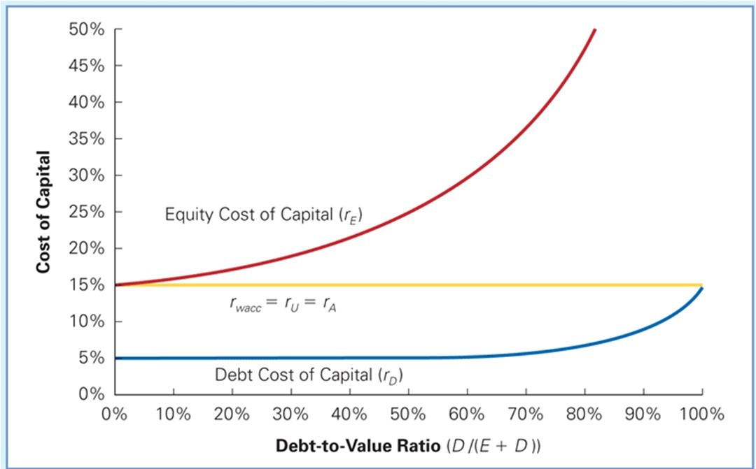
If a firm is levered, project $R_A$ is equal to the firm’s weighted average cost of capital.

\[R_{wacc} = R_u = R_a\]

That is, with perfect capital markets, a firm’s WACC is independent of its capital structure and is equal to its equity cost of capital if it is unlevered, which matches the cost of capital of its assets.

14.3 MM II

Assuming taxes do not exist:

14.3 MM II

The takeaway:

Although debt has a lower cost of capital than equity, leverage does not lower a firm’s WACC. As a result, the value of the firm’s free cash flow evaluated using the WACC does not change, and so the enterprise value of the firm does not depend on its financing choices.

14.3 MM II

Problem

Honeywell International Inc. (HON) has a market debt−equity ratio of 0.5.

Assume its current debt cost of capital is 6.5%, and its equity cost of capital is 14%.

If HON issues equity and uses the proceeds to repay its debt and reduce its debt−equity ratio to 0.4, it will lower its debt cost of capital to 5.75%.

With perfect capital markets, what effect will this transaction have on HON’s equity cost of capital and WACC?

14.3 MM II

Current WACC

\[R_{wacc} = \frac{E}{E+D} \times R_e + \frac{D}{E+D} \times R_d = \frac{2}{2+1} \times 14 + \frac{1}{2+1} \times 6.5 = 11.5\%\]

New Cost of Equity:

\[R_e = R_u + \frac{D}{E} (R_u - R_a) = 11.5 +0.4 \times (11.5 - 5.75) = 13.8\%\]

“New” WACC:

\[R_{wacc_{new}} = \frac{1}{1+0.4} \times 13.8 + \frac{0.4}{1+0.4} \times 5.75 = 11.5\%\]

Multiple Securities

If the firm’s capital structure is made up of multiple securities, then the WACC is calculated by computing the weighted average cost of capital of all of the firm’s securities.

Let’s say the firm has Equity (E), Debt (D), Warrant (W) issued:

\[R_{wacc} = R_u = R_e \times \frac{E}{E+D+W} + R_d \times \frac{D}{E+D+W} + R_w \times \frac{W}{E+D+W} \]

Levered and unlevered Betas

Remember that

\[\beta_u = \frac{E}{D+E} \times \beta_e + \frac{D}{D+E} \times \beta_d\]

When a firm changes its capital structure without changing its investments, its unlevered beta will remain unaltered. However, its equity beta will change to reflect the effect of the capital structure change on its risk.

\[\beta_e = \beta_u + \frac{D}{E} (\beta_u - \beta_d)\]

Obs

Unlevered Beta: A measure of the risk of a firm as if it did not have leverage, which is equivalent to the beta of the firm’s assets.

Levered and unlevered Betas

Problem

In August 2018, Reenor had a market capitalization of 140 billion. It had debt of 25.4 billion as well as cash and short−term investments of 60.4 billion. Its equity beta was 1.09 and its debt beta was approximately zero. What was Reenor’s enterprise value at time? Given a risk−free rate of 2% and a market risk premium of 5%, estimate the unlevered cost of capital of Reenor’s business.

Reenor’s net debt = 25.4 − 60.4 billion = −35.0 billion. Enterprise value 140 billion − 35billion = 105 billion.

\[\beta_u = \frac{E}{E+D} \times \beta_e + \frac{D}{E+D} \times \beta_d = \frac{140}{105} \times 1.09 + \frac{-35}{105} \times 0 = 1.45\] Unlevered cost of capital:

\[R_u = 2\% + 1.45 \times 5\% = 9.25\%\]

14.4 Capital Structure Fallacies

We will discuss now two fallacies concerning capital structure:

Leverage increases earnings per share (EPS), thus increase firm value
Issuing new equity will dilute existing shareholders, so debt should be issued

14.4 Capital Structure Fallacies

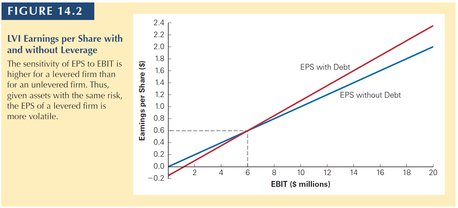
Leverage and EPS example

LVI is currently an all−equity firm.
It expects to generate earnings before interest and taxes (EBIT) of 10 million over the next year.
Currently, LVI has 10 million shares outstanding, and its stock is trading for a price of 7.50 per share.
LVI is considering changing its capital structure by borrowing 15 million at an interest rate of 8% and using the proceeds to repurchase 2 million shares at $7.50 per share.

Suppose LVI has no debt. Because there is no interest and no taxes, LVI’s earnings would equal its EBIT and LVI’s earnings per share without leverage would be

\[EPS=\frac{earnings}{Out. Shares}=\frac{10\;million}{10\;million}= 1\]

14.4 Capital Structure Fallacies

If LVI recapitalizes, the new debt will obligate LVI to make interest payments each year of $1.2 million/year
- 15 million × 8% interest/year = 1.2 million/year
As a result, LVI will have expected earnings after interest of 8.8 million
- Earnings = EBIT − Interest
- Earnings = 10 million − 1.2 million = 8.8 million

\[EPS=\frac{earnings}{Out. Shares}=\frac{8.8\;million}{8\;million}= 1.1\] EPS increases. Should firm value increase?

The answer is no.

Just like equity becomes riskier when the firm issues debt, the earnings stream is also riskier when the firm issues debt.

14.4 Capital Structure Fallacies

	(no debt)	(with debt)
EBIT	10	10
- Interets	0	1.2
Earnings	10	8.8
# shares (out)	10	10
EPS	1	1.1

14.4 Capital Structure Fallacies

No debt

EBIT	0	2	4	6	8	10	12	14	16	18	20
- Int.	0	0	0	0	0	0	0	0	0	0	0
Earnings	0	2	4	6	8	10	12	14	16	18	20
# shares	10	10	10	10	10	10	10	10	10	10	10
EPS	0	0.2	0.4	0.6	0.8	1	1.2	1.4	1.6	1.8	2.0

14.4 Capital Structure Fallacies

With debt

EBIT	0	2	4	6	8	10	12	14	16	18	20
- Int.	1.2	1.2	1.2	1.2	1.2	1.2	1.2	1.2	1.2	1.2	1.2
Earnings	-1.2	0.8	2.8	4.8	6.8	8.8	10.8	12.8	14.8	16.8	18.8
# shares	10	10	10	10	10	10	10	10	10	10	10
EPS	-0.12	0.08	0.28	0.48	0.68	0.88	1.08	1.28	1.48	1.68	1.88

14.4 Capital Structure Fallacies

Problem

Assume that LVI’s EBIT is not expected to grow in the future and that all earnings are paid as dividends. Use MM proposition I and II to show that the increase in expected EPS for LVI will not lead to an increase in the share price.

Solution

Without leverage, expected earnings per share and therefore dividends are 1 each year, and the share price 7.50. Let r be LVI’s cost of capital without leverage. Then we can value LVI as a perpetuity:

\[P = 7.50 = \frac{Div}{R_u} = \frac{EPS}{R_u} = \frac{1}{R_u}\]

Therefore, current stock price implies that $R_u = \frac{1}{7.50} = 13.33\%$

14.4 Capital Structure Fallacies

The market value of LVI without leverage is 7.50 × 10 million shares = 75 million.
If LVI uses debt to repurchase 15 million worth of the firm’s equity
then the remaining equity will be worth 75 million − 15million = 60 million.

After the transaction, $\frac{D}{E} = \frac{1}{4}$, thus, we can write:

\[R_e= R_u +\frac{D}{E} \times (R_u - R_d) = 13.33 + 0.25 \times (13.33 - 8) = 14.66\]

Given that expected EPS is now 1.10 per share, the new value of the shares equals

\[P=\frac{1.10}{14.66} = 7.50\]

Thus, even though EPS is higher, due to the additional risk, shareholders will demand a higher return. These effects cancel out, so the price per share is unchanged.

14.4 Capital Structure Fallacies

Because the firm’s earnings per share and price-earnings ratio are affected by leverage, we cannot reliably compare these measures across firms with different capital structures.

The same is true for accounting-based performance measures such as return on equity (ROE).

Therefore, most analysts prefer to use performance measures and valuation multiples that are based on the firm’s earnings before interest has been deducted.

For example, the ratio of enterprise value to EBIT (or EBITDA) is more useful when analyzing firms with very different capital structures than is comparing their P/E ratios.

14.4 Capital Structure Fallacies

Equity Issuances and Dilution

It is sometimes (incorrectly) argued that issuing equity will dilute existing shareholders’ ownership, so debt financing should be used instead.

Dilution: An increase in the total of shares that will divide a fixed amount of earnings

Suppose Jet Sky Airlines (JSA) currently has no debt and 500 million shares of stock outstanding, which is currently trading at a price of $16.

Last month the firm announced that it would expand and the expansion will require the purchase of $1 billion of new planes, which will be financed by issuing new equity.

The current (prior to the issue) value of the equity and the assets of the firm is 8 billion.
- 500 million shares × 16 per share = 8 billion

14.4 Capital Structure Fallacies

Suppose now JSA sells 62.5 million new shares at the current price of 16 per share to raise the additional 1 billion needed to purchase the planes.

Assets	Before	After
Cash		1000
Existing assets	8000	8000
Total Value	8000	9000
# shares (out)	500	562.5
Value per share	16	16

Result: share prices don’t change. Any gain or loss associated with the transaction will result from the NPV of the investments the firm makes with the funds raised.

14.5 MM: Beyond the Propositions

MM is truly about the Conservation of Value Principle in perfect financial markets

With perfect capital markets, financial transactions neither add nor destroy value
They only represent a repackaging of risk (and therefore return).
This implies that any financial transaction that appears to be a good deal may be exploiting some type of market imperfection.

Now it is your turn…

Interact

Remember to solve:

Interact

THANK YOU!

QUESTIONS?

Henrique C. Martins