Estratégia Financeira

Part 4 - ch.12 Estimating the Cost of Capital

Henrique C. Martins

10-03-2024

Chapter Outline

12.1 The Equity Cost of Capital

12.2 The Market Portfolio

12.3 Beta Estimation

12.4 The Debt Cost of Capital

12.5 A Project’s Cost of Capital

12.6 Project Risk Characteristics and Financing

12.7 Final Thoughts on Using the CAPM

12.1 The Equity Cost of Capital

The CAPM Equation for the Cost of Capital (using the Security Market Line).

The cost of capital of any investment opportunity equals the expected return of available investments with the same beta.

\[R_i = R_f + \beta \times (E[R_m] - R_f)\]

12.1 The Equity Cost of Capital

Problem

Suppose you estimate that Disney’s stock (DIS) has a volatility of 20% and a beta of 1.29. A similar process for Chipotle (CMG) yields a volatility of 30% and a beta of 0.55.

Which stock carries more total risk? Which has more market risk?

Disney has more Systematic risk.

Chipotle has more total risk.

12.1 The Equity Cost of Capital

Problem

If the risk-free interest rate is 3% and you estimate the market’s expected return to be 8%, calculate the equity cost of capital for DIS and CMG. Which company has a higher cost of equity capital?

\[R_{DIS}=3\%+1.29 \times (8\%−3\%) = 3\% + 6.45\% =9.45\%\]

\[R_{GMG}=3\%+0.55 \times(8\%−3\%)=3\%+2.75\%=5.75\%\]

Because market risk cannot be diversified, it is market risk that determines the cost of capital; thus DIS has a higher cost of equity capital than CMG, even though it is less volatile.

12.1 The Equity Cost of Capital

Suppose you estimate that Walmart’s stock has a volatility of 16.1% and a beta of 0.20. A similar process for Johnson & Johnson yields a volatility of 13.7% and a beta of 0.54. Which stock carries more total risk? Which has more market risk?

Walmart stock has more total risk.

Johnson & Johnson has a higher beta, so it has more market risk

12.1 The Equity Cost of Capital

If the risk-free interest rate is 4% and you estimate the market’s expected return to be 12%, calculate the equity cost of capital for Walmart and Johnson & Johnson. Which company has a higher cost of equity capital?

\[r_{JNJ}=4\%+0.54×(12\%−4\%)=4\%+4.32\%=8.32\%\]

\[r_{WMT}=4\%+0.20×(12\%−4\%)=4\%+1.6\%=5.6\%\]

Because market risk cannot be diversified, it is market risk that determines the cost of capital; thus, Johnson & Johnson has a higher cost of equity capital than Walmart, even though it is less volatile.

12.2 The Market Portfolio

To use the CAPM, we need to understand what the market portfolio is.

Because the market portfolio is the total supply of securities, the proportions of each security should correspond to the proportion of the total market that each security represents.

Thus, the market portfolio contains more of the largest stocks and less of the smallest stocks.

Market capitalization (of one firm):

The total market value of a firm’s outstanding shares

\[MV_i = (nr\;of\;shares\;outstanding) \times (price\;per\;share) = N_i \times P_i\]

12.2 The Market Portfolio

We then calculate the portfolio weights of each security: that is a Value-Weighted Portfolio

A portfolio in which each security is held in proportion to its market capitalization

\[x_i = \frac{MV_i}{Total\; MV}= \frac{MV_i}{\sum{MV}}\]

12.2 The Market Portfolio

Passive portfolio

trade not often

Active portfolio

trade often

12.2 The Market Portfolio

Examples of indexes:

SP500: A value-weighted portfolio of the 500 largest U.S. stocks
Dow Jones Industrial Average (DJIA): A price-weighted portfolio of 30 large industrial stocks (holds an equal number of shares of each stock).
Ibov : Around 90 BR stocks. Follows an algorithm focusing on liquidity.

ETFs (Exchange-traded funds): A portfolio that follows an index, like the SP500.

SP500 and Ibov are not considered as the market portfolio, they are proxies for the market portfolios. I.e., reasonable approximations.

R
Python

stocks <-c('SPY', 'IVV','VOO', 'SPLG' , '^GSPC') 
start <-'2010-01-01' 
end   <-Sys.Date()  
data <- yf_get(tickers = stocks, 
                         first_date = start,
                         last_date = end)
data<-data[complete.cases(data),] 
stock1 <- subset(data, ticker == stocks[1])
stock2 <- subset(data, ticker == stocks[2])
stock3 <- subset(data, ticker == stocks[3])
stock4 <- subset(data, ticker == stocks[4])
stock5 <- subset(data, ticker == stocks[5])
stock1$price_close2 <- stock1$price_close  / stock1$price_close[1] * 100
stock2$price_close2 <- stock2$price_close  / stock2$price_close[1] * 100
stock3$price_close2 <- stock3$price_close  / stock3$price_close[1] * 100
stock4$price_close2 <- stock4$price_close  / stock4$price_close[1] * 100
stock5$price_close2 <- stock5$price_close  / stock5$price_close[1] * 100
data2 <- rbind(stock1, stock2, stock3, stock4, stock5)
p<-ggplot(data2, aes(ref_date , price_close2, color=ticker))+
        geom_line() +
        labs(x = "",
             y='Closing prices', 
             title="SP500 against 4 ETFs, Initial price = 100", 
             subtitle = "Begin 01/01/2010") +   theme_solarized()
ggplotly(p)

Python

import matplotlib.pyplot as plt
import numpy as np
import pandas as pd
import yfinance as yf
stocks = ['SPY', 'IVV', 'VOO', 'SPLG', '^GSPC']
start = '2010-01-01'
end = pd.Timestamp.now()
data = yf.download(stocks, start=start, end=end)['Close']
## 
[                       0%                       ]
[*******************   40%                       ]  2 of 5 completed
[**********************60%****                   ]  3 of 5 completed
[**********************80%*************          ]  4 of 5 completed
[*********************100%***********************]  5 of 5 completed
data2 = (data / data.iloc[0]) * 100
plt.close()
plt.plot(data2)
plt.xlabel('')
plt.ylabel('Closing prices')
plt.title('SP500 against 4 ETFs, Initial price = 100\nBegin 01/01/2010')
plt.legend(data2.columns)
plt.show()

R
Python

stocks <-c('BOVA11.SA', '^BVSP') 
start <-'2010-01-01' 
end   <-Sys.Date()  
data <- yf_get(tickers = stocks, 
                         first_date = start,
                         last_date = end)
data<-data[complete.cases(data),] 
stock1 <- subset(data, ticker == stocks[1])
stock2 <- subset(data, ticker == stocks[2])
stock1$price_close2 <- stock1$price_close  / stock1$price_close[1] * 100
stock2$price_close2 <- stock2$price_close  / stock2$price_close[1] * 100
data2 <- rbind(stock1, stock2)
p<- ggplot(data2, aes(ref_date , price_close2, color=ticker))+
        geom_line() +
        labs(x = "",
             y='Closing prices', 
             title="IBOV against 2 ETFs, Initial price = 100", 
             subtitle = "Begin 01/01/2010") +   theme_solarized(base_size = 12) 
ggplotly(p)

Python

stocks = ['BOVA11.SA', '^BVSP']
start = '2010-01-01'
end = pd.Timestamp.now()
data = yf.download(stocks, start=start, end=end)['Close']
## 
[                       0%                       ]
[*********************100%***********************]  2 of 2 completed
data2 = (data / data.iloc[0]) * 100
plt.close()
plt.plot(data2)
plt.xlabel('')
plt.ylabel('Closing prices')
plt.title('Ibov against 2 ETFs, Initial price = 100')
plt.legend(data2.columns)
plt.show()

12.2 The Market Portfolio

Another key ingredient of CAPM is The Market Risk Premium

Risk-Free Rate
- The yield on U.S. Treasury securities
- Surveys suggest most practitioners use 10- to 30-year treasuries
- Highest quality assets
- Often, we use a short-term risk-free rate to evaluate a short-term investment, and a long-term rate when evaluating a long-term investment.
- In Brazil, Selic for the short-term. Or maybe a more suitable long-term fixed rate, like 20-30 years.

12.2 The Market Portfolio

The Historical Risk Premium
- Estimate the risk premium ($E[R_M] − R_f$) using the historical average excess return of the market over the risk-free interest rate
- Notice that, even with long periods, we often have large standard errors
- Also, implicitly, you are assuming that the past is a good proxy for the future.

R
Python

url <- "https://ceqef.fgv.br/sites/default/files/2023-12/Serie%20de%20Equity%20Risk%20Premium%20Novembro%20de%202023.xlsx"
download(url, dest="files/epr.xlsx", mode="wb") 
data <- read_excel("files/epr.xlsx", col_types = c("date","numeric") )
data <- data[2:nrow(data),1:2]
colnames(data) <- c("month", "erp")

p<-ggplot(data, aes(x=month, y = erp)) + geom_line() + theme_solarized()+
  labs(y = "Equity Risk Premium (ERP)", 
       x = "", 
       title = "Equity Risk Premium (ERP) in Brazil" , 
       caption = "Source: https://ceqef.fgv.br/node/594" )
ggplotly(p)

Python

import pandas as pd
import matplotlib.pyplot as plt
url = "https://ceqef.fgv.br/sites/default/files/2023-12/Serie%20de%20Equity%20Risk%20Premium%20Novembro%20de%202023.xlsx"
data = pd.read_excel(url, header=2)
data = data.iloc[:, 0:2]
data.columns = ["month", "erp"]
fig, ax = plt.subplots(figsize=(20, 10))
ax.plot(data["month"], data["erp"])
ax.set_xlabel("Time", fontsize=20)
ax.set_ylabel("Equity Risk Premium (ERP)", fontsize=20)
ax.set_title("Equity Risk Premium (ERP) in Brazil", fontsize=25)
ax.text(0.5, -0.1, "Source: https://ceqef.fgv.br/node/594", transform=ax.transAxes, ha="center")
plt.show()

12.2 The Market Portfolio

Using historical data has two problems:

Standard errors of the estimates are often large
They are backward looking

So, one alternative is to use the discount rate that is consistent with the current level of the index.

\[ R_m = \frac{Div_1}{P_o} + g = Dividend\; yield + Expected\; dividend\; growh\; rate\]

Let’s say, Ibov’s current dividend yield is 2%. Also, both earnings and dividends per share are expected to grow 6% per year.

\[ R_m = Dividend\; yield + Expected\; dividend\; growh\; rate = 2\% + 6\% = 8\%\]

12.3 Beta Estimation

Finally, we need to estimate Beta

Recall, beta is the expected percent change in the excess return of the security for a 1% change in the excess return of the market portfolio.
At the end of the day, Beta is the coefficient of a linear regression

In the following examples, Beta of Petr is around 1.1, while the Beta of Wege is around 0.45.

R
Python

freq.data   <- 'daily'
start <-'2000-01-01' 
end   <-Sys.Date()  
ibov <- yf_get(tickers = "^BVSP",
                        first_date = start,
                        last_date = end,
                        thresh_bad_data = 0.5,
                        freq_data = freq.data)
asset <- yf_get(tickers = "PETR4.SA",
                        first_date = start,
                        last_date = end,
                        thresh_bad_data = 0.5,
                        freq_data = freq.data )
ret_ibov <- ibov  %>% tq_transmute(select = price_adjusted,
                                   mutate_fun = periodReturn,
                                   period = 'daily',
                                   col_rename = 'return',
                                   type = 'log')
ret_asset <- asset   %>%tq_transmute(select = price_adjusted,
                                     mutate_fun = periodReturn,
                                     period = 'daily',
                                     col_rename = 'return',
                                     type = 'log')
ret <- left_join(ret_ibov, ret_asset, by = c("ref_date" = "ref_date"))
window <-252
ret$var <- roll_cov(ret$return.x, ret$return.x, width = window)
ret$cov <- roll_cov(ret$return.x, ret$return.y, width = window)
ret$beta <- ret$cov / ret$var
ret <- subset(ret, ret$beta != "NA" )
p<-ggplot(ret, aes(x= return.x, y=return.y)) + 
  geom_point()+
  geom_smooth(method=lm, se=FALSE)+
  labs( y = "Daily returns PETR4", x="Daily returns IBOV",title = "Beta PETR4")+
  xlim(-0.2, 0.2) + ylim(-0.2, 0.2) +   theme_solarized()
ggplotly(p)

Python

stocks = ['PETR4.SA', '^BVSP']
start = '2010-01-01'
end = pd.Timestamp.now()
data = yf.download(stocks, start=start, end=end)['Close']
returns = data.pct_change().dropna()
plt.close()
fig, ax = plt.subplots(figsize=(20, 10))
ax.scatter(returns["^BVSP"], returns["PETR4.SA"], alpha=0.5, color='black')
m, b = np.polyfit(returns["^BVSP"], returns["PETR4.SA"], 1)
ax.plot(returns["^BVSP"], m*returns["^BVSP"] + b, color='darkblue')
ax.set_xlabel("Daily returns IBOV")
ax.set_ylabel("Daily returns PETR4")
ax.set_title("Beta PETR4")
ax.set_xlim(-0.2, 0.2)
ax.set_ylim(-0.2, 0.2)
plt.show()

R
Python

ibov <- yf_get(tickers = "^BVSP",
                        first_date = start,
                        last_date = end,
                        thresh_bad_data = 0.5,
                        freq_data = freq.data )
asset <- yf_get(tickers = "WEGE3.SA",
                        first_date = start,
                        last_date = end,
                        thresh_bad_data = 0.5,
                        freq_data = freq.data )
ret_ibov <- ibov  %>%tq_transmute(select = price_adjusted,
                                  mutate_fun = periodReturn,
                                  period = 'daily',
                                  col_rename = 'return',
                                  type = 'log')
ret_asset <- asset %>%tq_transmute(select = price_adjusted,
                                  mutate_fun = periodReturn,
                                  period = 'daily',
                                  col_rename = 'return',
                                  type = 'log')
ret <- left_join(ret_ibov, ret_asset, by = c("ref_date" = "ref_date"))
window <-252
ret$var <- roll_cov(ret$return.x, ret$return.x, width = window)
ret$cov <- roll_cov(ret$return.x, ret$return.y, width = window)
ret$beta <- ret$cov / ret$var
ret <- subset(ret, ret$beta != "NA" )
p<-ggplot(ret, aes(x= return.x, y=return.y)) + 
  geom_point()+
  geom_smooth(method=lm, se=FALSE)+
  labs( y = "Daily returns WEGE3", x="Daily returns IBOV",title = "Beta WEGE3")+
  xlim(-0.2, 0.2) + ylim(-0.2, 0.2) +   theme_solarized()
ggplotly(p)

Python

stocks = ['WEGE3.SA', '^BVSP']
start = '2010-01-01'
end = pd.Timestamp.now()
data = yf.download(stocks, start=start, end=end)['Close']
returns = data.pct_change().dropna()
plt.close()
fig, ax = plt.subplots(figsize=(20, 10))
ax.scatter(returns["^BVSP"], returns["WEGE3.SA"], alpha=0.5, color='black')
m, b = np.polyfit(returns["^BVSP"], returns["WEGE3.SA"], 1)
ax.plot(returns["^BVSP"], m*returns["^BVSP"] + b, color='darkblue')
ax.set_xlabel("Daily returns IBOV")
ax.set_ylabel("Daily returns WEGE3")
ax.set_title("Beta WEGE3.SA")
ax.set_xlim(-0.2, 0.2)
ax.set_ylim(-0.2, 0.2)
plt.show()

12.3 Beta Estimation

Note that in any period, the asset’s returns can be higher or lower than the best-fitting line.
Such deviations from the best-fitting line result from risk that is not related to the market as a whole.
These deviations are zero on average in the graph, as the points above the line balance out the points below the line.
They represent firm-specific risk that is diversifiable and that averages out in a large portfolio.

12.3 Beta Estimation

We can estimate Beta using the following regression:

\[(R_i - R_f) = \alpha_i + \beta_i \times (R_m - R_f) + \epsilon_i\]

$\epsilon_i$ is the error term or the residual. It represents the deviation from the best-fitting line and is zero on average (or else we could improve the fit). This error term corresponds to the diversifiable risk of the stock, which is the risk that is uncorrelated with the market.

12.3 Beta Estimation

$\alpha_i$ is the constant term. It measures the historical performance of the security relative to the expected return predicted by the security market line.
It is the distance that the stock’s average return is above or below the SML. Thus, we can say $\alpha_i$ is a risk-adjusted measure of the stock’s historical performance.
According to the CAPM, $\alpha_i$ should not be significantly different from zero.

12.3 Beta Estimation

Finally, we can estimate Beta using the formula (use market s.d. = 10%):

\[Beta_i = \frac{Sd(R_i) \times Corr(R_i,R_m)}{Sd(R_m)} = \frac{Cov(R_i,R_m)}{Var(R_m)}\]

Portfolio	Weight	Volatility (Sd)	Correlation with M
HEC Corp	0.21	13%	0.42
Green Midget	0.31	20%	0.68
Alive And Well	0.48	12%	0.54

$Beta_{H} = \frac{Sd(R_i) \times Corr(R_i,R_m)}{Sd(R_m)} = \frac{0.13 \times 0.42}{0.10} = 0.546$
$Beta_{G} = \frac{Sd(R_i) \times Corr(R_i,R_m)}{Sd(R_m)} = \frac{0.20 \times 0.68}{0.10} = 1.36$
$Beta_{A} = \frac{Sd(R_i) \times Corr(R_i,R_m)}{Sd(R_m)} = \frac{0.12 \times 0.54}{0.10} = 0.648$

12.3 Beta Estimation

Problem

Suppose you have estimated Tikyberd’s beta to be 0.8 with a 95% confidence interval of 0.65 to 0.95.

Assuming the risk-free rate is 2% and the market is expected to return 12%, what range would you estimate for Tikyberd’s equity cost of capital?

\[E[R_i]=r_f + β_i (E[R_M] −R_f) =2\% + 0.65 (12\% − 2\%) = 8.5\%\]

\[E[R_i]=r_f + β_i (E[R_M] −R_f) = 2\% + 0.95 (12\% − 2\%) = 11.5\%\]

12.4 The Debt Cost of Capital

Let’s discuss now how to calculate the cost of debt.

Debt Yields Versus Returns

Yield to maturity is the IRR an investor will earn from holding the bond to maturity and receiving its promised payments.
If there is little risk the firm will default, yield to maturity is a reasonable estimate of investors’ expected rate of return.
- If there is significant risk of default, yield to maturity will overstate investors’ expected return.

12.4 The Debt Cost of Capital

Table 12.2 shows average annual default rates by debt rating, as well as the peak default rates experienced during recessionary periods.

12.4 The Debt Cost of Capital

Assume that the average loss rate for unsecured debt is 60%.

According to Table 12.2, during average times the annual default rate for B-rated bonds is 5.5%.

So the expected return to B-rated bondholders during average times is 0.055 × 0.60 = 3.3% below the bond’s quoted yield.

\[R_d = YTM - default \;rate \times average\; loss\; rate \]

12.4 The Debt Cost of Capital

Debt Betas

We can also use the CAPM to estimate debt cost.
But we will need the debt beta.
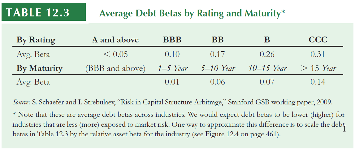
Debt betas are difficult to estimate because corporate bonds are traded infrequently.
One approximation is to use estimates of betas of bond indices by rating category.

12.4 The Debt Cost of Capital

Problem

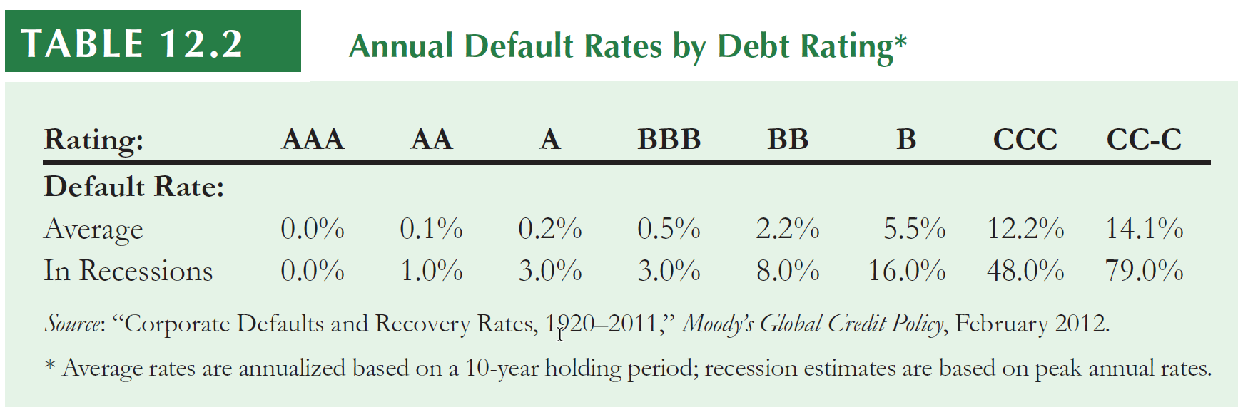
In early 2013, auto parts retailer Autozone had outstanding 10-year bonds with a yield to maturity of 3% and a BBB rating. If corresponding risk-free rates were 1.5% and the market risk premium is 8%, estimate the expected return of Autozone’s debt.

Solution I

Using the average estimates in Table 12.2 and an expected loss rate of 60%, from Eq. 12.7 we have

\[R_d = 3\% - 0.5\% \times 0.6 = 2.7\%\]

Solution II

Alternatively, we can estimate the bond’s expected return using CAPM and an estimated beta of 0.10 from Table 12.3.

In that case, $R_d = 1.5\% + 0.10(8\%) = 2.3\%$.

12.4 The Debt Cost of Capital

Both estimates are rough approximations and they both suggest that the expected return of Autozone’s debt is below its yield-to-maturity of 3%.

12.5 A Project’s Cost of Capital

We want now to estimate the cost of capital of a project.

Because a new project is not itself a publicly traded security, we cannot use historical risks of equity and debt to estimate beta and the cost of capital.

Also, the decision to invest in projects using the firm’s cost of capital might ignore the project’s risk.

12.5 A Project’s Cost of Capital

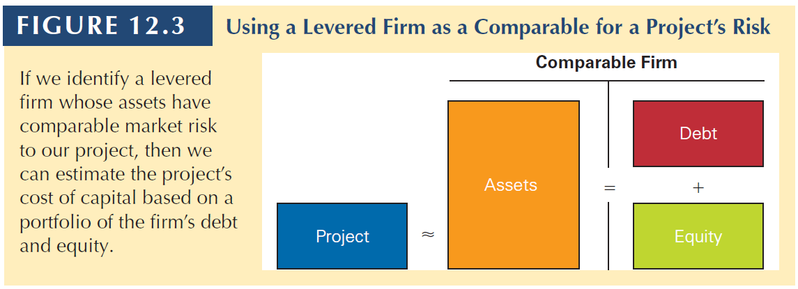
Instead, the most common method for estimating a project’s beta is to identify comparable firms in the same line of business as the project we are considering undertaking.

All-Equity Comparables

The simplest setting of a theoretical comparable firm is to find an all-equity financed firm (a firm with no debt) in a single line of business that is comparable to the project.

Then, use the comparable firm’s equity beta and cost of capital as estimates.

The main idea here is that your project is an asset, so if you find an all-equity firm, the equity beta will also be the beta of its assets. Thus, you can use this estimate as the beta of your project.

Remember that:

Assets = Equity + Debt.
When debt is zero: Assets = Equity.

12.5 A Project’s Cost of Capital

Equity beta: the one we measured before.

Asset beta: it is the beta of all assets in a firm, which is the same beta of the combination of Equity + Debt.

Debt beta: the changes in the expected return by 1% change in the market returns.

If your project is comparable to the assets of a firm, you can use its beta as your project’s beta.

But again, the firm might be all-equity or might have debt.

12.5 A Project’s Cost of Capital

Estimating the Beta of a Project from a Single-Product Firm

Problem

You have just invented a new low-cost, long-lasting rechargeable battery for use in electric cars.

You are working on your business plan, and believe your firm will face similar market risk to Seguin Inc, which has a beta of 1.3.

To develop your financial plan, estimate the cost of capital of financing your firm assuming a risk-free rate of 2.5% and a market risk premium of 6.5%.

Using Seguin’s beta as the estimate of the project beta (i.e., assuming the market risk of your project is the same as this company’s):

\[R_{project} = 2.5\% + 1.3 \times 6.5\% = 10.95\%\]

This will be the cost of capital of your project.

12.5 A Project’s Cost of Capital

Things get more complex in levered firms.

For levered firms, Assets = Equity + Debt.
So, the cash flows generated by the firm’s assets are used to pay both debt and equity holders.
As a result, the returns of the firm’s equity alone are not representative of the underlying assets.
In fact, because of debt, equity will often be much riskier.
Thus, the beta of a levered firm’s equity will not be a good estimate of the beta of its assets and of our project.

12.5 A Project’s Cost of Capital

In order to compute the cost of capital of such a project and assuming the comparable firm has debt, you need to unlever the comparable firm’s beta.

Asset cost of capital = unlevered cost of capital
is the expected return required by the firm’s investors to hold the firm’s underlying assets

Asset or unlevered cost of capital:

\[R_u = \frac{E}{E+D}\times R_e + \frac{D}{E+D} \times R_d\]

12.5 A Project’s Cost of Capital

Because the beta of a portfolio is the weighted-average of the betas:

\[\beta_u = \frac{E}{E+D}\times \beta_e + \frac{D}{E+D} \times \beta_d\]

12.5 A Project’s Cost of Capital

Problem

Your firm is launching a new product and you identify Company X as a firm with comparable investments.

X’s equity has a market capitalization of 77 billion and a beta of 0.75. X also has 57 billion of AA-rated debt outstanding, with an average yield of 4.1%.

Estimate the cost of capital of your firm’s investment given a risk-free rate of 2.5% and a market risk-premium of 6%.

Company’s X equity cost of capital is:

\[ R_e = 2.5\% + 0.75 \times 6\% = 7\%\]

Company’s X unlevered cost of capital is (using the yield as debt cost):

\[R_u =\frac{77}{77+57} \times 7\% + \frac{57}{77+57} \times 4.1\% = 5.76\%\]

12.5 A Project’s Cost of Capital

Problem

We can also use X’s unlevered Beta and CAPM.

Assuming debt beta = 0:

\[\beta_u =\frac{77}{77+57} \times 0.75 + \frac{57}{77+57} \times 0 = 0.43\]

\[ R_e = 2.5\% + 0,43 \times 6\% = 5.08\%\]

12.5 A Project’s Cost of Capital

Cash and Net Debt

Holding cash is a risk-free asset. It is a good idea to exclude cash holdings when computing the asset’s risk.

We can measure the Net debt:

\[Net \;debt = Debt - cash\; and \; ST \;investments\]

Also, remember the idea of enterprise value

\[Enterprise\; Value = Market \;Value \;of \;Equity + Debt - Cash\]

12.5 A Project’s Cost of Capital

Example

Apple’s market capitalization in mid-2016 was $484 billion, and its beta was 1.03. At that same time, the company had $25 billion in cash and $69 billion in debt. Based on this data, estimate the beta of Apple’s underlying business enterprise.

\[\beta_u = \frac{E}{E+D}\times \beta_e + \frac{D}{E+D} \times \beta_d = \frac{484}{484+69-25}\times 1.03 + \frac{69-25}{484+69-25} \times 0 = 0.944\]

Note that the firm is less risky than its equity portion due to its cash holdings.

12.5 A Project’s Cost of Capital

Industry Betas

Remember that estimating the beta of a stock only contains estimation error.

Instead, you can estimate the beta of a whole industry to reduce the estimate error.

12.6 Project Risk and Financing

In this final section, we want to account for risk differences between projects.

Individual projects may be more or less sensitive to market risk.

One important thing is that:

firm asset betas reflect the market risk of the average project in the firm.
But individually, projects can differ in risk.
For instance, think about a multi-divisional firm.
- Each division will likely have its own level of market risk.

12.6 Project Risk and Financing

Operating leverage

Additionally, operating leverage can also affect the project’s risk.

High operating leverage, high risk.

Operating leverage is the proportion of fixed costs over total costs.

A higher proportion of fixed costs increases the sensitivity of the project’s cash flows to market risk.

The project’s beta will be higher
A higher cost of capital should be assigned

12.6 Project Risk and Financing

Now, we have all that is necessary to compute the Weighted Average Cost of Capital (WACC).

Assuming the existence of Taxes:

\[R_{wacc} = \frac{E}{D+E}\times R_e + \frac{D}{D+E} \times R_d \times (1-\phi_c)\] This is the after-tax WACC.

Because interest expense is tax deductible, the WACC is less than the expected return of the firm’s assets. Meaning, you do not pay taxes on debt interests, which makes the after-tax WACC decrease in comparison to the pre-tax WACC

12.6 Project Risk and Financing

Pre-tax WACC

\[R_u = \frac{E}{E+D}\times R_e + \frac{D}{E+D} \times R_d\]

Expected return investors will earn by holding the firm’s assets
In a world with taxes, it can be used to evaluate an all-equity project with the same risk as the firm

After-tax WACC

\[R_{wacc} = \frac{E}{D+E}\times R_e + \frac{D}{D+E} \times R_d \times (1-\phi_c)\]

With taxes, WACC can be used to evaluate a project with the same risk and the same financing as the firm

12.6 Project Risk and Financing

Cavo Corp’s equity cost of capital is 15%, and its debt cost of capital is 7%.
The corporate tax rate is 34%.
The firm has 100 million in debt outstanding and a market capitalization of 250 million.
What is Cabo’s unlevered cost of capital?
What is Cavo’s weighted average cost of capital?

12.6 Project Risk and Financing

Unlevered cost of capital is:

\[R_u = \frac{250}{250+100}\times 15\% + \frac{100}{250+100} \times 7\% = 12.71\%\]

WACC is:

\[R_{wacc} = \frac{250}{250+100}\times 15\% + \frac{100}{250+100} \times 7\% \times (1-0,34) = 12,03\%\]

12.7 Final thoughts on using CAPM

CAPM is very practical and straightforward to implement, the CAPM-based approach is very robust
CAPM imposes a disciplined process on managers to identify the cost of capital.
CAPM make the capital budgeting process less subject to managerial manipulation than if managers could set project costs of capital without clear justification.
CAPM is often the model many investors use to evaluate risk.
CAPM gets managers to think about risk in the correct way. That is, to think about market risk, instead of total risk.

Now it is your turn…

Practice

Remember to solve:

Interact

THANK YOU!

QUESTIONS?

Henrique C. Martins