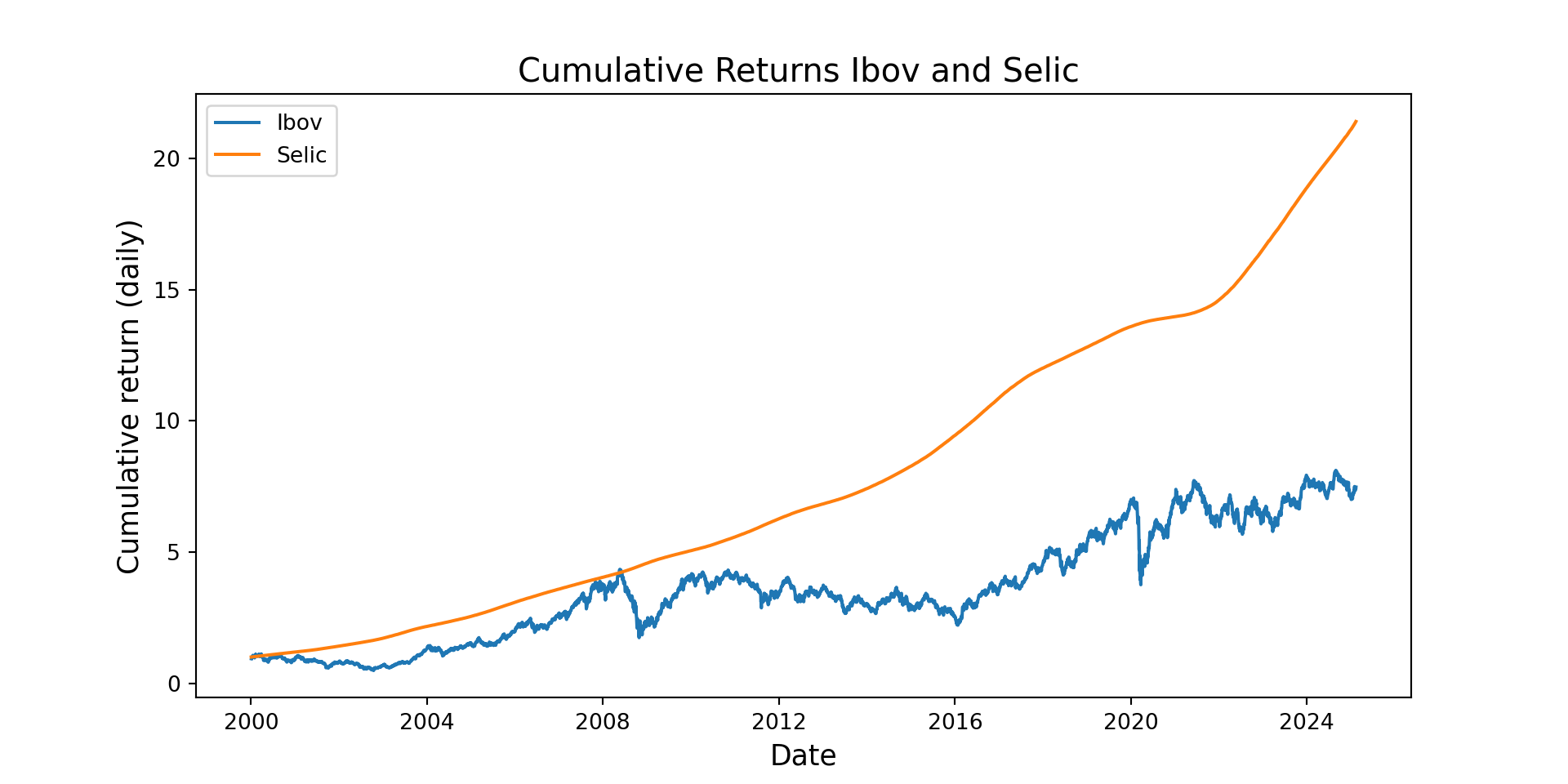
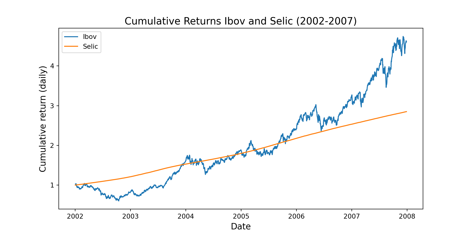
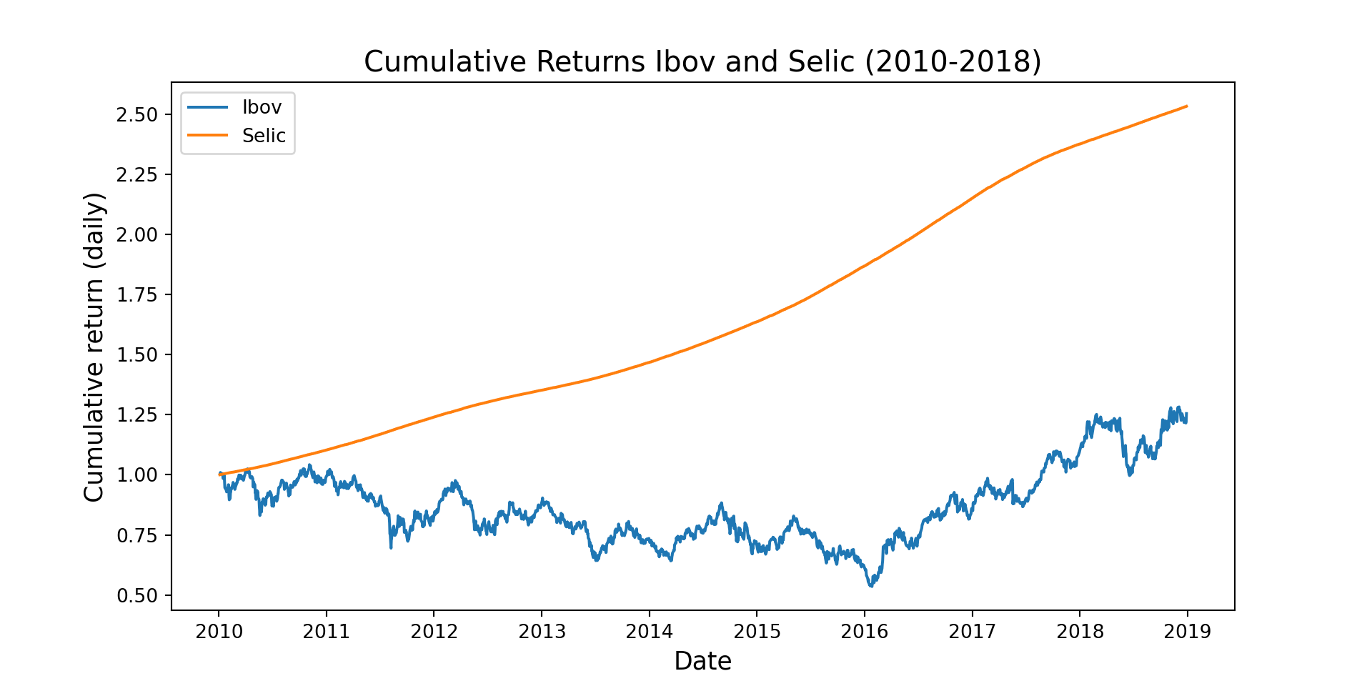
library(downloader)library(dplyr)library(GetQuandlData)library(ggplot2)library(ggthemes)library(PerformanceAnalytics)library(plotly)library(readxl)library(roll)library(tidyr)library(tidyquant)library(yfR)# Ibovstock <-'^BVSP'start <-'2010-01-01'# Adjusted start dateend <-'2018-12-31'# Adjusted end dateibov <-yf_get(tickers = stock, first_date = start, last_date = end)ibov <- ibov[order(as.numeric(ibov$ref_date)),]# Cumulative return Ibovibov$Ibov_return <- ibov$cumret_adjusted_prices -1# Selic - Download manually from ipeadata "Taxa de juros: Overnight / Selic"selic <-read_excel("files/selic.xls")names(selic) <-c("ref_date", "selic")selic$ref_date <-as.Date(selic$ref_date, format ="%d/%m/%Y")selic <-na.omit(selic)selic$selic <- selic$selic / (252*100)# Filter Selic data for the desired period (2010-2020)selic <- selic %>%filter(ref_date >= start & ref_date <= end)# Cumulative return Selicreturn_selic <-data.frame(nrow(selic):1)colnames(return_selic) <-"selic_return"for (i in (2:nrow(selic))) { return_selic[i, 1] <-Return.cumulative(selic$selic[1:i])}# Merging dataframesselic <-cbind(selic, return_selic)df <-merge(ibov, selic, by =c("ref_date"))df$selic_return[1] <-NAdf$Ibov_return[1] <-NA# Graph cumulated return CDI and IBOVp <-ggplot(df, aes(ref_date)) +geom_line(aes(y = Ibov_return, colour ="Ibov")) +geom_line(aes(y = selic_return, colour ="Selic")) +labs(y ='Cumulative return (daily)') +theme_solarized() +ggtitle("Cumulative Returns Ibov, and Selic (2010-2018)")ggplotly(p)
Python
# Define API key and other parametersimport matplotlib.pyplot as pltimport pandas as pdimport yfinance as yfstock ="^BVSP"start ="2010-01-01"end ="2018-12-31"# Get data for IBOVibov = yf.download(stock, start=start, end=end)ibov = ibov.reset_index()ibov = ibov.sort_values("Date")ibov = ibov.rename(columns={'Date': 'ref_date', 'Adj Close': 'Ibovespa'})ibov["return"] = ibov["Ibovespa"].pct_change()ibov['Ibov_return'] = (1+ ibov['return']).cumprod()ibov = ibov[['ref_date', 'Ibov_return']]# Get data for Selicselic = pd.read_excel("files/selic.xls")selic.columns = ["ref_date", "selic"]selic['ref_date'] = pd.to_datetime(selic['ref_date'], format="%d/%m/%Y")selic = selic.dropna()selic['selic'] = selic['selic'] / (252*100)# Filter Selic data for the desired periodselic = selic[(selic['ref_date'] >= start) & (selic['ref_date'] <= end)]# Calculate cumulative return for Selicselic['selic_return'] = (1+ selic['selic']).cumprod()# Merge dataframesdf = pd.merge(ibov, selic, on="ref_date")# Plot datafig, ax = plt.subplots(figsize=(10,5))ax.plot(df["ref_date"], df["Ibov_return"], label='Ibov')ax.plot(df["ref_date"], df["selic_return"], label='Selic')plt.ylabel('Cumulative return (daily)', fontsize=13)plt.title('Cumulative Returns Ibov and Selic (2010-2018)', fontsize=15)plt.xlabel('Date', fontsize=13)plt.legend(loc='upper left')plt.show()
10.2 Measures of Risk and Return
10.2 Measures of Risk and Return
When an investment is risky, it may earn different returns.
Each possible return has some likelihood of occurring.
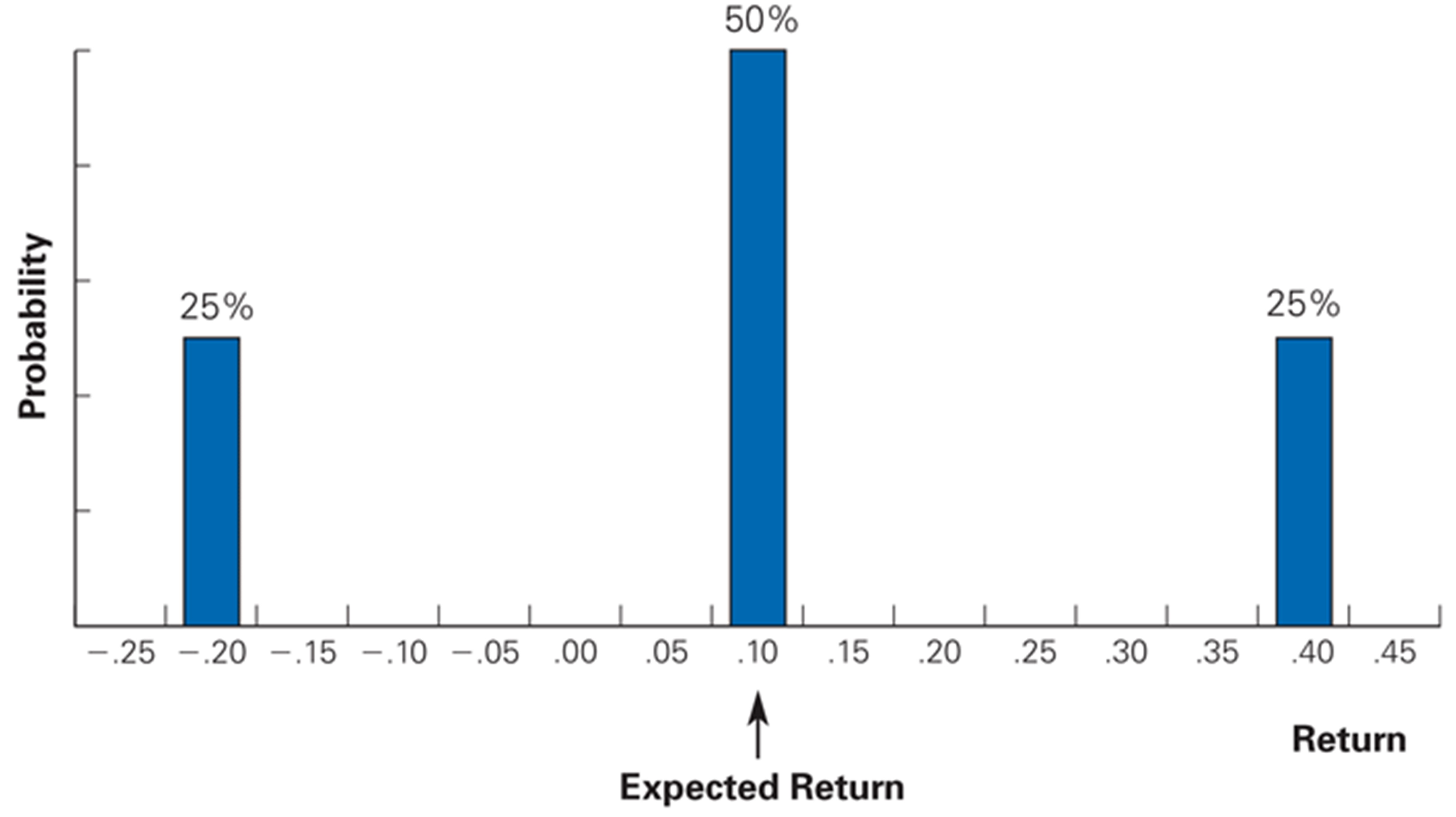
This information is summarized with a probability distribution, which assigns a probability, \(P_r\) , that each possible return, \(R\), will occur.
Assume BFI stock currently trades for 100 per share. In one year, there is a 25% chance the share price will be 140, a 50% chance it will be 110, and a 25% chance it will be 80.
10.2 Measures of Risk and Return
This insight will lead to this kind of graph.
10.2 Measures of Risk and Return
Let’s see how to compute the expected return on this asset.
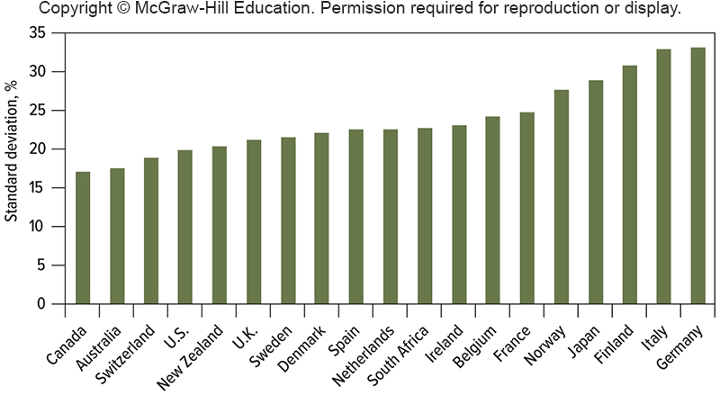
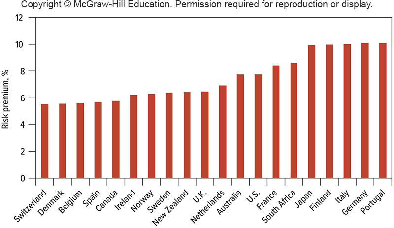
Keep in mind: There is variation (heterogeneity) in the level of standard deviation across countries.
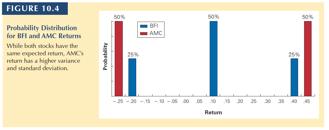
Source: Brealey, Myers and Allen (13ed)
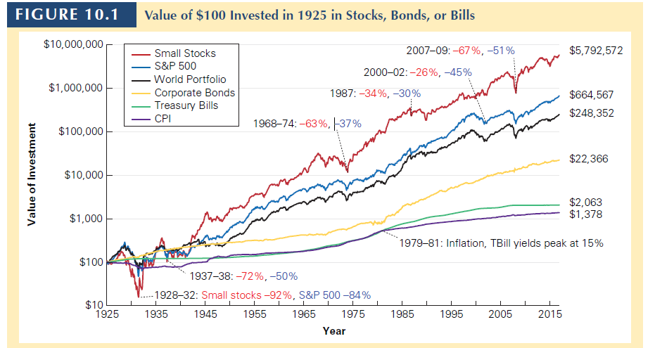
10.3 Historical Returns
10.3 Historical Returns
The previous problem was a simple one-time-ahead example (i.e., we computed the expected return one period ahead).
A more realistic one is to compute historical returns:
\[R_{t+1} = \frac{Div_{t+1} + P_{t+1}}{P_t} - 1\]
This is:
Dividend Yield + Capital Gain Rate
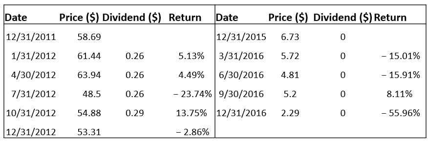
10.3 Historical Returns
Calculating realized annual returns
If a stock pays dividends at the end of each quarter (with realized returns RQ1, RQ2, RQ3, and RQ4 each quarter), then its annual realized return, \(R_{annual}\), is computed as follows:
Warning: because you are using a sample of historical returns (instead of the population) there is a T-1 in the variance formula.
10.3 Historical Returns
Historical Returns: standard error
We can use a security’s historical average return to estimate its actual expected return. However, the average return is just an estimate of the expected return.
Standard Error
A statistical measure of the degree of estimation error of a statistical estimate
The average return is just an estimate of the true expected return, and is subject to estimation error.
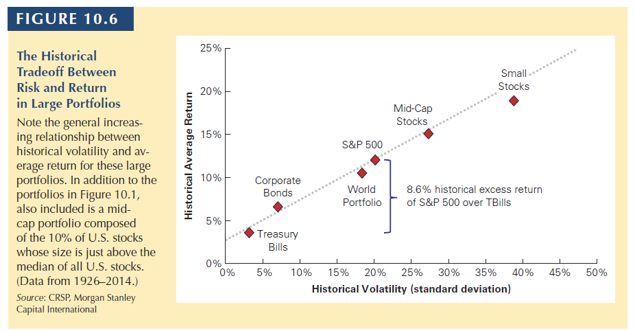
For example, from 1926 to 2017 the average return of the S&P 500 was 12.0% with a volatility of 19.8%.
\[E[R] \pm 2\times SE = 12\% \pm \frac{19.8\%}{\sqrt{92}}= 12\% \pm 4.1\%\]This means that, with 95% confidence interval, the expected return of the S&P 500 during this period ranges from 7.9% and 16.1%.
The longer the period, the more accurate you are. But even with 92 years of data, you are not very accurate to predict the expected return of the SP500.
10.3 Historical Returns
Some analysts prefer to use a geometric average instead of arithmetic average.
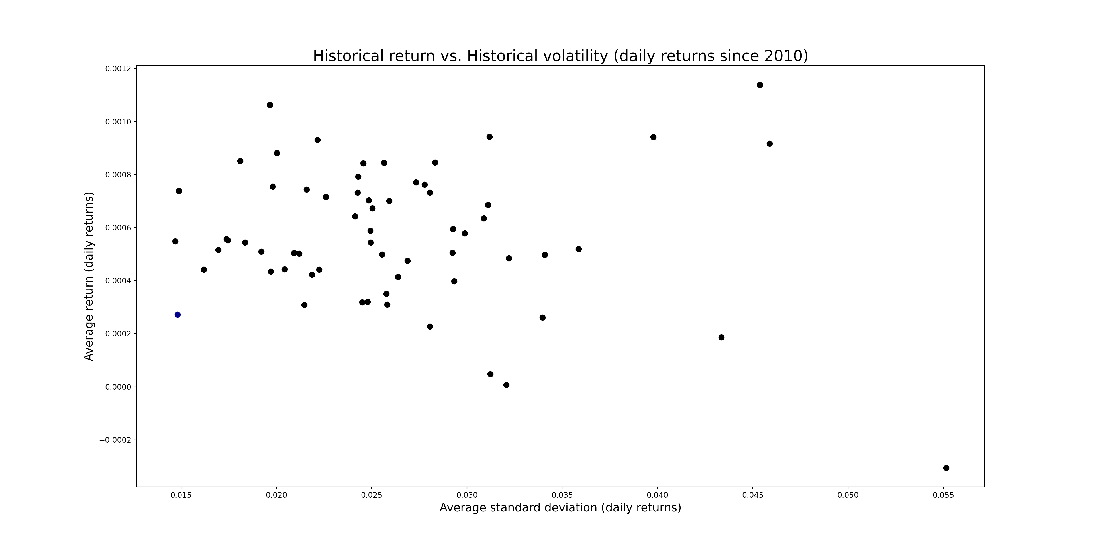
start ='2010-01-01'end = pd.Timestamp.now()stocks = ["^BVSP","ABEV3.SA","ALPA4.SA","AMER3.SA","B3SA3.SA","BBAS3.SA","BBDC3.SA","BBDC4.SA","BEEF3.SA","BPAN4.SA","BRAP4.SA","BRFS3.SA","BRKM5.SA","BRML3.SA","CCRO3.SA","CIEL3.SA","CMIG4.SA","COGN3.SA","CPFE3.SA","CPLE6.SA","CSAN3.SA","CSNA3.SA","CYRE3.SA","DXCO3.SA","ECOR3.SA","EGIE3.SA","ELET3.SA","ELET6.SA","EMBR3.SA","ENBR3.SA","ENEV3.SA","ENGI11.SA","EQTL3.SA","EZTC3.SA","FLRY3.SA","GGBR4.SA","GOAU4.SA","GOLL4.SA","HYPE3.SA","ITSA4.SA","ITUB4.SA","JBSS3.SA","JHSF3.SA","LREN3.SA","MGLU3.SA","MRFG3.SA","MRVE3.SA","MULT3.SA","PCAR3.SA","PETR3.SA","PETR4.SA","PRIO3.SA","QUAL3.SA","RADL3.SA","RENT3.SA","SANB11.SA","SBSP3.SA","SULA11.SA","SUZB3.SA","TAEE11.SA","TIMS3.SA","TOTS3.SA","UGPA3.SA","USIM5.SA","VALE3.SA","VIIA3.SA","VIVT3.SA","WEGE3.SA","YDUQ3.SA"]results = []for ticker in stocks: asset = yf.download(ticker, start=start, end=end) asset['return'] = asset['Adj Close'].pct_change() asset = asset.dropna() mean_return = asset['return'].mean() std_return = asset['return'].std() data = pd.DataFrame({'ticker': [ticker], 'average_return': [mean_return], 'standard_deviation': [std_return]}) results.append(data)df = pd.concat(results).reset_index(drop=True)plt.close()fig, ax = plt.subplots(figsize=(20, 10))for i inrange(len(df)):if df.loc[i, 'ticker'] =='^BVSP': color ='darkblue'else: color ='black' ax.scatter(x=df.loc[i, 'standard_deviation'], y=df.loc[i, 'average_return'], s=50, color=color)plt.title("Historical return vs. Historical volatility (daily returns since 2010)", fontsize=20)plt.xlabel("Average standard deviation (daily returns)", fontsize=15)plt.ylabel("Average return (daily returns)", fontsize=15)plt.show()
10.6 Diversification
10.6 Diversification
When you have a portfolio containing assets, the risk you incurred is less than the (weighted average) of the assets’ risk. Let’s understand why.
First, we need to separate two types of risk:
Firm-specific risk (or news):
good or bad news about the company itself. For example, a firm might announce that it has been successful in gaining market share within its industry.
this type of risk is independent across firms.
also called firm-specific, idiosyncratic, unique, or diversifiable risk.
Market-wide risk (or news):
news about the economy as a whole, affects all stocks. For instance, changes in the interest rates.
this type of risk is common to all firms.
also called systematic, undiversifiable, or market risk.
10.6 Diversification
Firm-Specific Versus Systematic Risk
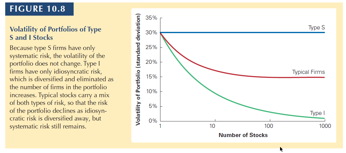
When many stocks are combined in a large portfolio, the firm-specific risks for each stock will average out and be diversified. The systematic risk, however, will affect all firms and will not be diversified.
Consider two types of firms:
Type S firms are affected only by systematic risk. There is a 50% chance the economy will be strong and they will earn a return of 40%. There is a 50% change the economy will be weak and their return will be −20%. Because all these firms face the same systematic risk, holding a large portfolio of type S firms will not diversify the risk.
Type I firms are affected only by firm-specific risks. Their returns are equally likely to be 35% or −25%, based on factors specific to each firm’s local market. Because these risks are firm specific, if we hold a portfolio of the stocks of many type I firms, the risk is diversified.
10.6 Diversification
You must be aware that actual firms are affected by both market-wide risks and firm-specific risks.
When firms carry both types of risk, only the unsystematic risk will be diversified when many firm’s stocks are combined into a portfolio.
The volatility will therefore decline until only the systematic risk remains.
That is why the standard deviation of a portfolio (like Ibov) is lower than the weighted average standard deviation of the stocks in it. It is like free lunch.
1) it occurs only if the risk of the stocks are independent
we will define later what “independent” means to us.
intuitively, different firms have different risks.
2) if the risks are independent, more stocks means less risk…
… until a certain point.
10.6 Diversification
Consider again type I firms, which are affected only by firm-specific risk. Because each individual type I firm is risky, should investors expect to earn a risk premium when investing in type I firms?
The risk premium for diversifiable risk is zero, so investors are not compensated for holding firm-specific risk.
The reason is that they can mitigate this part of risk through diversification.
Diversification eliminates this risk for free, implying that all investors should have a diversified portfolio. Otherwise, the investor is not rational.
The takeaway is:
The risk premium of a security is determined by its systematic risk and does not depend on its diversifiable risk.
10.6 Diversification
In a world where diversification exists:
Standard deviation is not a good measure for risk anymore.
Standard deviation is a measure of a stock’s total risk
But if you are diversified, you are not incurring the total risk, only the systematic risk.
We will need a measure of a stock’s systematic risk.
This measure is called: Beta
But make no mistake:
The standard deviation of the returns of a portfolio is still a good measure for the portfolio’s risk!
But you will not use the average standard deviation of individual stocks contained in a portfolio.
10.7 Measuring Systematic Risk
10.7 Measuring Systematic Risk
Beta
To measure the systematic risk of a stock, determine how much of the variability of its return is due to systematic risk versus unsystematic risk.
To determine how sensitive a stock is to systematic risk, look at the average change in the return for each 1% change in the return of a portfolio that fluctuates solely due to systematic risk.
This is the exact definition of a Beta in a regression or a linear relationship (we studied that in statistics).
Saying the same thing in other words:
Beta measures the expected percent change in the excess return of a security for a 1% change in the excess return of the market portfolio.
Market portfolio contains all stocks: SP500 is a proxy, Ibov is another (for BR).
10.7 Measuring Systematic Risk
Suppose the market portfolio tends to increase by 47% when the economy is strong and decline by 25% when the economy is weak. What is the beta of a type S firm whose return is 40% on average when the economy is strong and −20% when the economy is weak?
Firm S
Market changes 47%, stock changes 40%: Beta is \(\frac{40}{47}=0.85\)
Market changes -25%, stock changes -20%: Beta is \(\frac{20}{25}=0.8\)
Market changes from -25% to 47% = 72%, stock changes from -20 to 40, Beta is \(\frac{60}{72}=0.833\)
It does not mean that the stock has three betas…
… it means that we have three estimates for the stock’s beta.
10.7 Measuring Systematic Risk
Suppose the market portfolio tends to increase by 47% when the economy is strong and decline by 25% when the economy is weak. What is the beta of a type S firm whose return is 40% on average when the economy is strong and −20% when the economy is weak? What is the beta of a type I firm that bears only idiosyncratic, firm-specific risk?
Firm I
Does not change, Beta is \(\frac{0}{72}=0\)
Market Risk Premium
We can define: The market risk premium is the reward investors expect to earn for holding a portfolio with a beta of 1.
\[Market\; risk\;premium = E[R_m] - R_{rf}\]
Inverting:
\[E[R_m] = R_{rf} + Market\; risk\;premium\]
The idea is that investors are risk-averse and dislike risk. Therefore, in order to invest in risky assets, investors demand an extra return.
Flipping the argument, a risky asset will have to pay an extra return for its additional risk in order to attract investors.
Therefore, there is a clear association between the risk and return of assets.
Again: in a diversified portfolio, investors are diversified so they only worry about beta (not standard deviation).
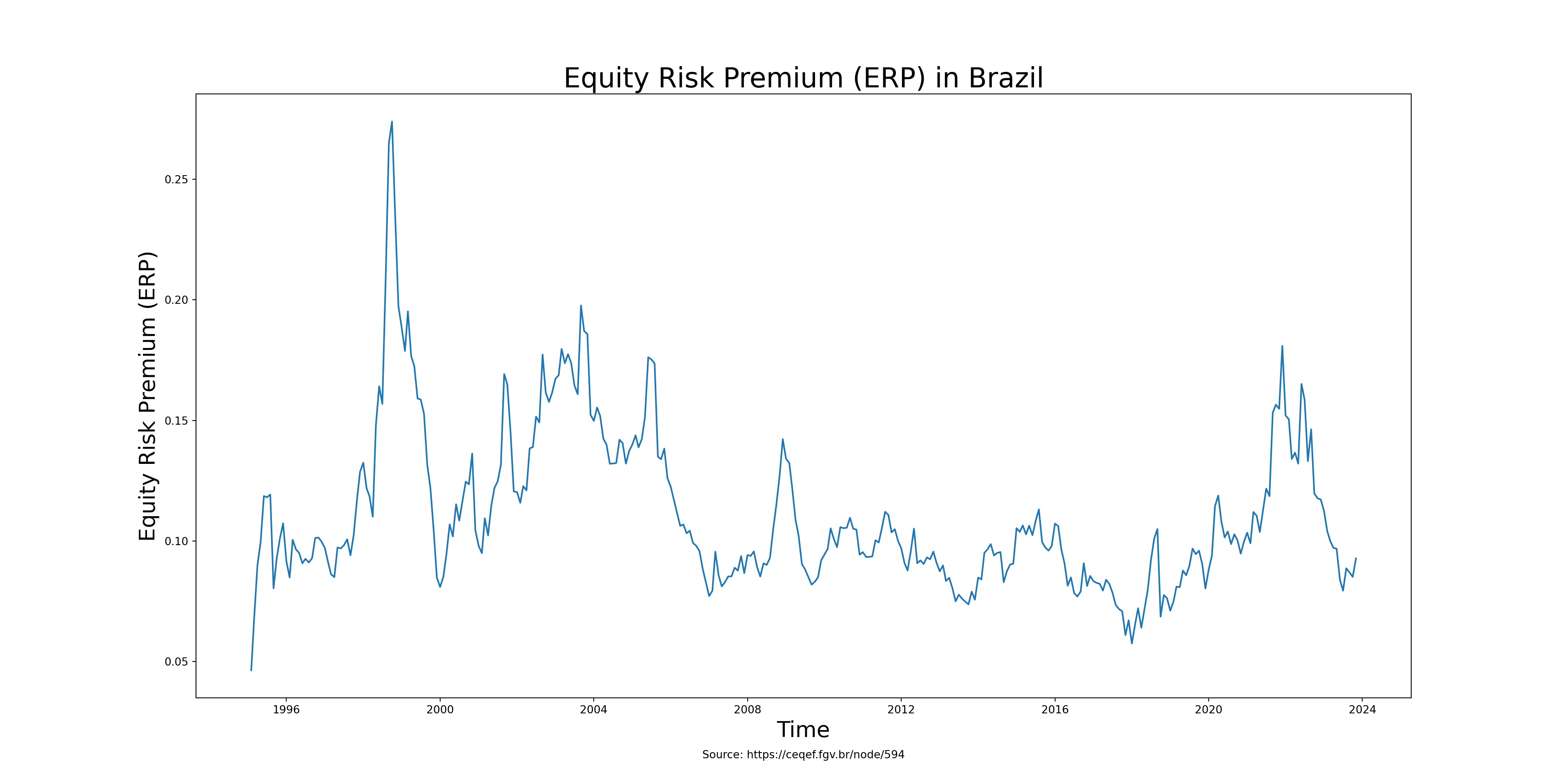
Market Risk Premium
There is some heterogeneity in the risk premium across countries.
Assume the economy has a 60% chance that the market return will be 15% next year and a 40% chance the market return will be 5% next year. Assume the risk-free rate is 6%. If a company’s beta is 1.18, what is its expected return next year?