Estratégia Financeira

Module 2 - ch.10 Capital Markets and the Pricing of Risk

Henrique C. Martins

18-08-2025

⚠️ Disclaimer – Virtual HCM Responses

The Virtual HCM is powered by AI to assist you with course materials.
While it is trained on the course’s content, it may occasionally:

• Misinterpret the question or context.
  
• Generate inaccurate or incomplete information.
  
• Provide answers not explicitly included in the materials.

Your responsibility:
Always cross-check the answers with the book, slides, readings, and feedback provided in the course. In case you are not sure, ask the instructor.

💡 Use Virtual HCM as a learning aid, not as the sole source of truth.

Ranking tokens

These actions count toward your participation grade.

• flash_quiz_participate — Submitted a quiz attempt on the slide. (+1)

• answer_correct_numeric — Correct numeric answer (within tolerance of 0.1). (+2)
• answer_wrong_numeric — Incorrect numeric answer. (0)

• answer_correct_long — Long-form answer manually graded as correct. (+5)
• answer_submitted_long — Submitted a long-form answer (recorded as not correct). (0)

• answer_correct_tf — Correct answer to a T/F question. (+1)
• answer_wrong_tf — Incorrect answer to a T/F question. (0)

• answer_correct_mcq — Correct answer to a MCQ. (+1)
• answer_wrong_mcq — Incorrect answer to a MCQ. (0)

• exit_ticket — Submitted the end-of-class reflection (Check-out). (+1)

• got_it — Reacted with a “Got it” to a slide. (+1)

Chapter outline

10.1 Risk and Return: Insights from History

10.2 Common Measures of Risk and Return

10.3 Historical Returns of Stocks and Bonds

10.4 The Historical Trade-Off Between Risk and Return

10.6 Diversification in Stock Portfolios

10.7 Measuring Systematic Risk

10.8 Beta and the Cost of Capital

10.1 Risk & Return: Insights

10.1 Risk & Return: Insights

10.1 Risk & Return: Insights

Some Insights:

• Small stocks had the highest long-term return, while T-Bills had the lowest.

• Small stocks had the largest fluctuations in price, while T-Bills had the lowest.

  • Higher risk requires a higher return.

• But, few people ever make an investment for so many years.

• More realistic investment horizons and different initial investment dates can greatly influence each investment’s risk and return.

Notice the volatility next slide.

10.1 Risk & Return: Insights

Insights from Brazil

library(downloader)
library(dplyr)
library(GetQuandlData)
library(ggplot2)
library(ggthemes)
library(PerformanceAnalytics)
library(plotly)
library(readxl)
library(roll)
library(tidyr)
library(tidyquant)
library(yfR)

#Ibov
stock<-'^BVSP' 
start<-'2000-01-01' 
end   <- Sys.Date() 
ibov <- yf_get(tickers = stock,first_date = start,last_date = end)
ibov<- ibov[order(as.numeric(ibov$ref_date)),]
# Cumulative return Ibov
ibov$Ibov_return <- ibov$cumret_adjusted_prices -1

#Selic - Download manually from ipeadata "Taxa de juros: Overnight / Selic"
selic <- read_excel("../files/selic.xls")
names(selic) <- c("ref_date", "selic")
selic$ref_date <- as.Date(selic$ref_date , format = "%d/%m/%Y")
selic <- na.omit(selic)
selic$selic <- selic$selic / (252* 100)

# Cumulative return Selic
return_selic <- data.frame(selic_return = rep(NA, nrow(selic)))
colnames(return_selic)<- "selic_return"
for(i in (2:nrow(selic))) {
return_selic[i,1] <- Return.cumulative( selic$selic[1:i] )
}

# Merging dataframes
selic <- cbind(selic, return_selic)
df <- merge(ibov ,selic, by=c("ref_date"))
df$selic_return[1] <- NA
df$Ibov_return[1] <- NA
# Graph cumulated return CDI and IBOV
p <- ggplot(df, aes(ref_date)) +
geom_line(aes(y = Ibov_return, colour = "Ibov")) +
geom_line(aes(y = selic_return, colour = "Selic")) +
labs(y='Cumulative return (daily)') + theme_solarized() +
  ggtitle("Cumulative Returns  Ibov, and Selic")
ggplotly(p)

Insights from Brazil (2002-2007).

library(downloader)
library(dplyr)
library(GetQuandlData)
library(ggplot2)
library(ggthemes)
library(PerformanceAnalytics)
library(plotly)
library(readxl)
library(roll)
library(tidyr)
library(tidyquant)
library(yfR)

# Ibov
stock <- '^BVSP'
start <- '2002-01-01'  # Adjusted start date
end <- '2007-12-31'   # Adjusted end date
ibov <- yf_get(tickers = stock, first_date = start, last_date = end)
ibov <- ibov[order(as.numeric(ibov$ref_date)),]

# Cumulative return Ibov
ibov$Ibov_return <- ibov$cumret_adjusted_prices - 1

# Selic - Download manually from ipeadata "Taxa de juros: Overnight / Selic"
selic <- read_excel("../files/selic.xls")
names(selic) <- c("ref_date", "selic")
selic$ref_date <- as.Date(selic$ref_date, format = "%d/%m/%Y")
selic <- na.omit(selic)
selic$selic <- selic$selic / (252 * 100)

# Filter Selic data for the desired period (2010-2020)
selic <- selic %>% filter(ref_date >= start & ref_date <= end)

# Cumulative return Selic
return_selic <- data.frame(nrow(selic):1)
colnames(return_selic) <- "selic_return"
for (i in (2:nrow(selic))) {
  return_selic[i, 1] <- Return.cumulative(selic$selic[1:i])
}

# Merging dataframes
selic <- cbind(selic, return_selic)
df <- merge(ibov, selic, by = c("ref_date"))
df$selic_return[1] <- NA
df$Ibov_return[1] <- NA

# Graph cumulated return CDI and IBOV
p <- ggplot(df, aes(ref_date)) +
  geom_line(aes(y = Ibov_return, colour = "Ibov")) +
  geom_line(aes(y = selic_return, colour = "Selic")) +
  labs(y = 'Cumulative return (daily)') + theme_solarized() +
  ggtitle("Cumulative Returns Ibov, and Selic (2002-2007)")
ggplotly(p)

Insights from Brazil (2010-2018).

library(downloader)
library(dplyr)
library(GetQuandlData)
library(ggplot2)
library(ggthemes)
library(PerformanceAnalytics)
library(plotly)
library(readxl)
library(roll)
library(tidyr)
library(tidyquant)
library(yfR)

# Ibov
stock <- '^BVSP'
start <- '2010-01-01'  # Adjusted start date
end <- '2018-12-31'   # Adjusted end date
ibov <- yf_get(tickers = stock, first_date = start, last_date = end)
ibov <- ibov[order(as.numeric(ibov$ref_date)),]

# Cumulative return Ibov
ibov$Ibov_return <- ibov$cumret_adjusted_prices - 1

# Selic - Download manually from ipeadata "Taxa de juros: Overnight / Selic"
selic <- read_excel("../files/selic.xls")
names(selic) <- c("ref_date", "selic")
selic$ref_date <- as.Date(selic$ref_date, format = "%d/%m/%Y")
selic <- na.omit(selic)
selic$selic <- selic$selic / (252 * 100)

# Filter Selic data for the desired period (2010-2020)
selic <- selic %>% filter(ref_date >= start & ref_date <= end)

# Cumulative return Selic
return_selic <- data.frame(nrow(selic):1)
colnames(return_selic) <- "selic_return"
for (i in (2:nrow(selic))) {
  return_selic[i, 1] <- Return.cumulative(selic$selic[1:i])
}

# Merging dataframes
selic <- cbind(selic, return_selic)
df <- merge(ibov, selic, by = c("ref_date"))
df$selic_return[1] <- NA
df$Ibov_return[1] <- NA

# Graph cumulated return CDI and IBOV
p <- ggplot(df, aes(ref_date)) +
  geom_line(aes(y = Ibov_return, colour = "Ibov")) +
  geom_line(aes(y = selic_return, colour = "Selic")) +
  labs(y = 'Cumulative return (daily)') + theme_solarized() +
  ggtitle("Cumulative Returns Ibov, and Selic (2010-2018)")
ggplotly(p)

10.2 Measures of Risk and Return

10.2 Measures of Risk and Return

When an investment is risky, it may earn different returns.

Each possible return has some likelihood of occurring.

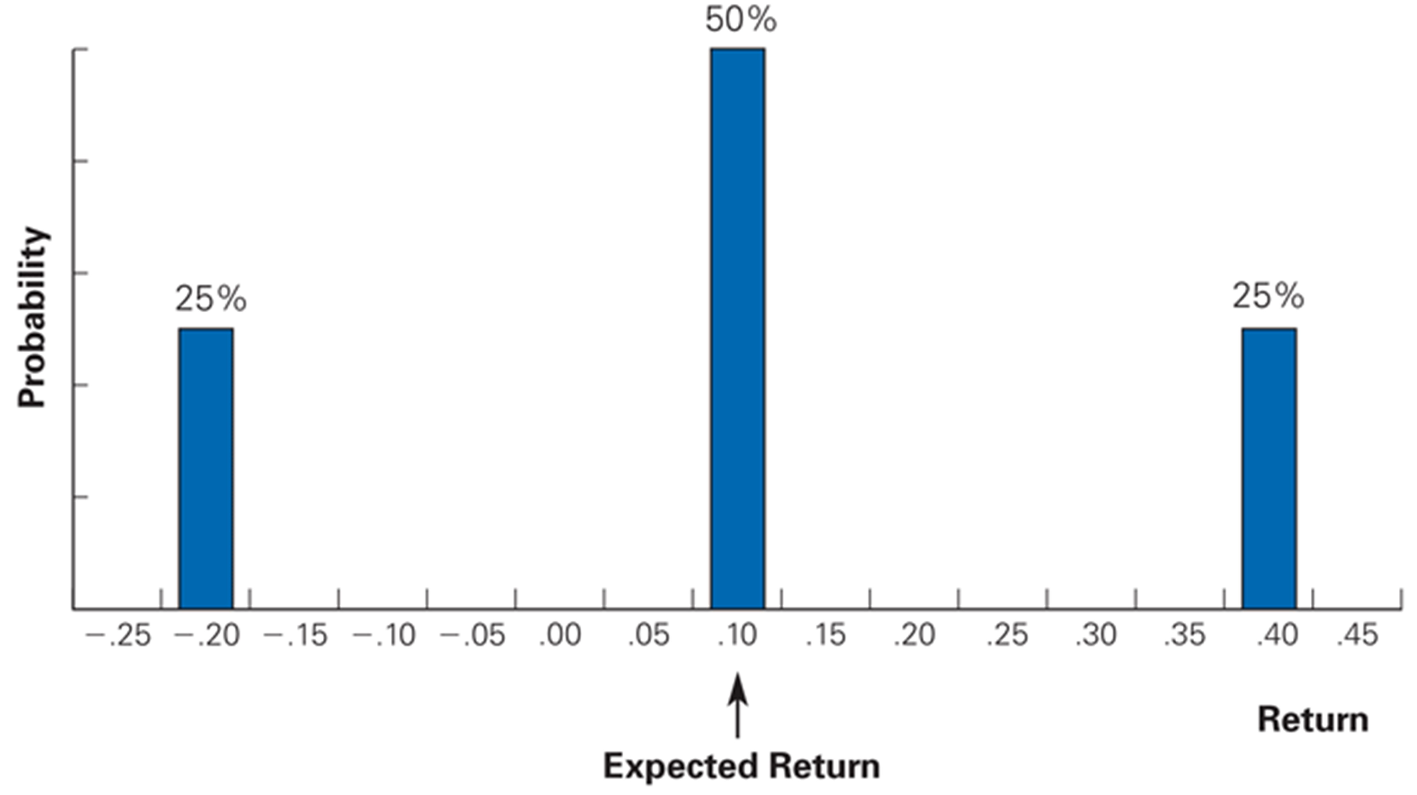
This information is summarized with a probability distribution, which assigns a probability, \(P_r\) , that each possible return, \(R\), will occur.

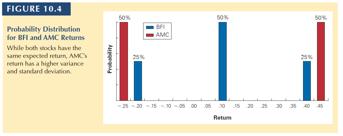
Assume BFI stock currently trades for 100 per share. In one year, there is a 25% chance the share price will be 140, a 50% chance it will be 110, and a 25% chance it will be 80.

10.2 Measures of Risk and Return

This insight will lead to this kind of graph.

10.2 Measures of Risk and Return

Let’s see how to compute the expected return on this asset.

\[Expected\;return = E[R] = \sum_{R} P_R \times R\]

\[E[R_{BFI}] = 25\%(−0.20) + 50\%(0.10) + 25\%(0.40) = 10\%\]

Very important: there is an underlying assumption that the past is good enough to teach us about the future.

That is, we are computing the historical average return and using this number as the best estimate of the expected return.

Keep that assumption in mind.

10.2 Measures of Risk and Return

Now risk: variance and standard deviation.

\[Var(R) = E[(R-E[R])^2] = \sum_{R} P_R \times (R-E[R])^2 \]

\[SD(R) = \sqrt{Var(R)}\]

\[V(R) = 0.25 × (−0.2 − 0.1)^2 + 0.5 × (0.1 − 0.1)^2 + 0.25 × (0.4 − 0.1)^2 = 0.045\]

\[SD(R_{BFI}) = \sqrt{0.045} = 21.2\%\]

10.2 Measures of Risk and Return

Suppose AMC stock is equally likely to have a 45% return or a −25% return. What are the expected return and volatility?

\[E[R] = 50\%×0.45+50\%×(−0.25)=10.0\%\]

\[Var[R] = 50\%×(0.45−0.10)^2+50\%×(−0.25−0.10)^2=0.1225\]

\[SD[R] = (0.1225) ^{0.5} = 35\%\]

10.2 Measures of Risk and Return

It is clear that riskier assets have heavier tails.

Warning: Standard deviation and variance are correct measures of total risk if the returns are normally distributed.

IBOV returns seem to follow a normal distribution.

stock <- '^BVSP'
start <- '2010-01-01'  # Adjusted start date
end <- Sys.Date()   # Adjusted end date
ibov <- yf_get(tickers = stock, first_date = start, last_date = end)
ibov <- ibov[order(as.numeric(ibov$ref_date)),]

# Cumulative return Ibov
ibov$Ibov_return <- ibov$cumret_adjusted_prices - 1

p<-ggplot(ibov,aes(ibov$ret_closing_prices))+
        geom_histogram(color='#006600',
                       bins = 100) + 
        labs(x = "",
             y='Daily return', 
             title="IBOV") +   theme_solarized()
ggplotly(p)

Standard deviation through time. It changes.

ibov$sd <- roll_sd(ibov$ret_closing_prices,  
                     width = 100,  
                     min_obs = 100 ) * sqrt(250)
p<-ggplot(ibov,aes(ref_date,sd))+
        geom_line(color='#2986cc') + 
        labs(x = "",
             y='Standard deviation using 100 daily returns', 
             title="IBOV (Daily returns since 2010)") +   theme_solarized()
ggplotly(p)

Standard deviation through time. Riskier is riskier.

stocks <-c('AMER3.SA' ) 
amer <- yf_get(tickers = stocks, 
                         first_date = start,
                         last_date = end)
amer<-amer[complete.cases(amer),]
amer$sd <- roll_sd(amer$ret_closing_prices,  
                     width = 100,  
                     min_obs = 100 ) * sqrt(250)
ibov <- subset(ibov, ref_date >= as.Date("2010-01-05"))

p<-ggplot() + 
  geom_line(data=amer, aes(ref_date, sd), color='#801e00') +
  geom_line(data=ibov, aes(ref_date, sd), color='#2986cc') +
          labs(x = "",y='Standard deviation using 100 daily returns', 
             title="IBOV vs AMER3 (Daily returns since 2010)") +   theme_solarized()
ggplotly(p)

Daily returns IBOV.

p<-ggplot(ibov,aes(ibov$ref_date,ibov$ret_closing_prices))+
        geom_line(color='#2986cc') + 
        labs(x = "",
             y='Daily returns', 
             title="IBOV (Daily returns since 2010)")   +   theme_solarized()  
ggplotly(p)

Daily returns Americanas.

p<-ggplot() +
  geom_line(data=amer, aes(amer$ref_date, amer$ret_closing_prices), color='#801e00') +
  geom_line(data=ibov, aes(ibov$ref_date, ibov$ret_closing_prices), color='#2986cc') +
  labs(x = "", y='Daily returns') +
  ggtitle("IBOV vs AMER3 (Daily returns since 2010)") +
  theme_solarized()
ggplotly(p)      

Americanas seems riskier than ITUB. Some stocks have heavier tails than others. The stock with the heavier tail is riskier.

stocks <-c('AMER3.SA', 'ITUB3.SA') 
start <-'2012-01-01' 
end   <- Sys.Date() 
data <- yf_get(tickers = stocks, 
                         first_date = start,
                         last_date = end)
data<-data[complete.cases(data),] 
p<-ggplot(data, aes(ret_closing_prices,  fill = ticker)) + 
        geom_histogram(bins = 100, alpha = 0.35, position='identity') + 
        labs(x = "",
             y='Daily returns', 
             title="Daily returns",
             subtitle = start)+
      xlim(-0.1,0.1) +   theme_solarized()
ggplotly(p)

10.3 Historical Returns

10.3 Historical Returns

The previous problem was a simple one-time-ahead example (i.e., we computed the expected return one period ahead).

A more realistic one is to compute historical returns:

\[R_{t+1} = \frac{Div_{t+1} + P_{t+1}}{P_t} - 1\]

This is:

Dividend Yield + Capital Gain Rate

10.3 Historical Returns

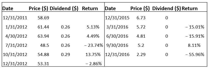
Calculating realized annual returns

If a stock pays dividends at the end of each quarter (with realized returns RQ1, RQ2, RQ3, and RQ4 each quarter), then its annual realized return, \(R_{annual}\), is computed as follows:

\[(1 + 𝑅_{annual}) = (1+𝑅_{Q1})\times(1+𝑅_{Q2})\times(1+ 𝑅_{Q3})\times (1+𝑅_{Q4})\]

• You can also compute using a daily time horizon (not manually, but by software).

One important piece of information you need:

• You should know whether the return is calculated adjusted by dividends (they usually are, but always ask).

10.3 Historical Returns

Compute the annual returns of this stock.

\[𝑅_{2012}=(1.0513)(1.0449)(0.7626)(1.1375)(0.9714)−1=−7.43\%\]

\[𝑅_{2016}=(0.8499)(0.8409)(1.0811)(0.440)−1=−66.0\%\]

Notice that the first example is not quarterly.

10.3 Historical Returns

Compute the annual returns of this stock.

Also notice that, since the firm did not pay dividends in 2016, you can compute:

\[\frac{2.29}{6.73}-1 = -66\%\]

10.3 Historical Returns

Some analysts prefer to use a geometric average instead of arithmetic average.

Also called Compound Annual Growth Rate (CAGR).

\[CAGR = [(1+R_1)\times(1+R_2)\times ...\times (1+R_T)]^{\frac{1}{T}}-1\]

\[CAGR = [\frac{Final\;value}{Initial\;value}]^\frac{1}{T}-1\]

Using Figure 10.1 of BM: geometric return of SP500 from 1926-2017 is

\[CAGR = [\frac{664,567}{100}]^\frac{1}{92}-1 = 10.04\%\]

Key: module2_slide1

• Return Breakdown
• Annual Returns
• CAGR

You bought a stock one year ago for $13.06 per share and sold it today for $12.61. It paid a $1.09 per share dividend today.

1. What was your realized return (in %)?

✅ Realized return = (p2 − p1 + div)/p1 × 100 = 4.97%.

2. What percentage of the return came from dividend yield?

✅ Dividend yield = div/p1 × 100 = 8.36%.

3. What percentage of the return came from capital gain?

✅ Capital gain = (p2 − p1)/p1 × 100 = -3.39%.

A stock paid quarterly dividends with realized returns: Q1: 2.59%, Q2: 2.21%, Q3: -0.61%, and Q4: 2.05%.

1. What was the annual realized return (in %)?

✅ Annual realized return = ((1+RQ1) × (1+RQ2) × (1+RQ3) × (1+RQ4) − 1) × 100 = 6.35%.

2. What is the simple average of the four quarterly returns (in %)?

✅ Simple average = (RQ1 + RQ2 + RQ3 + RQ4)/4 × 100 = 1.56%. The difference Annual realized return − Simple average = 4.79 p.p.

An investment grew from 88 to 151.18 over 8 years.

1. What is the CAGR (in %)? 

✅ Solution: CAGR = (()^{1/T} - 1). Here, (()^{1/8} − 1 = 7%.

Student ID:

Password:

10.3 Historical Returns

Average annual return

The average annual return of an investment during some historical period is simply the average of the realized returns for each year.

\[\tilde{R} = \frac{1}{T} (𝑅_1 + 𝑅_2 + ⋯ + 𝑅_𝑇) = \frac{1}{T} \sum_{t=1}^{T} R_t\]

Variance estimate using realized returns

\[Var[R] = \frac{1}{T-1} \sum_{t=1}^{T} (R_t- \tilde{R})^2 \] \[SD(R) = \sqrt{Var(R)}\]

Warning: because you are using a sample of historical returns (instead of the population) there is a T-1 in the variance formula.

10.3 Historical Returns

Historical Returns: standard error

We can use a security’s historical average return to estimate its actual expected return. However, the average return is just an estimate of the expected return.

• Standard Error
  • A statistical measure of the degree of estimation error of a statistical estimate

The average return is just an estimate of the true expected return, and is subject to estimation error.

You can compute the standard error as

\[SE = \frac{Standard\; deviation}{\sqrt{n\;of\; observations}}\]

10.3 Historical Returns

Historical Returns: standard error

Using BM p.367 example.

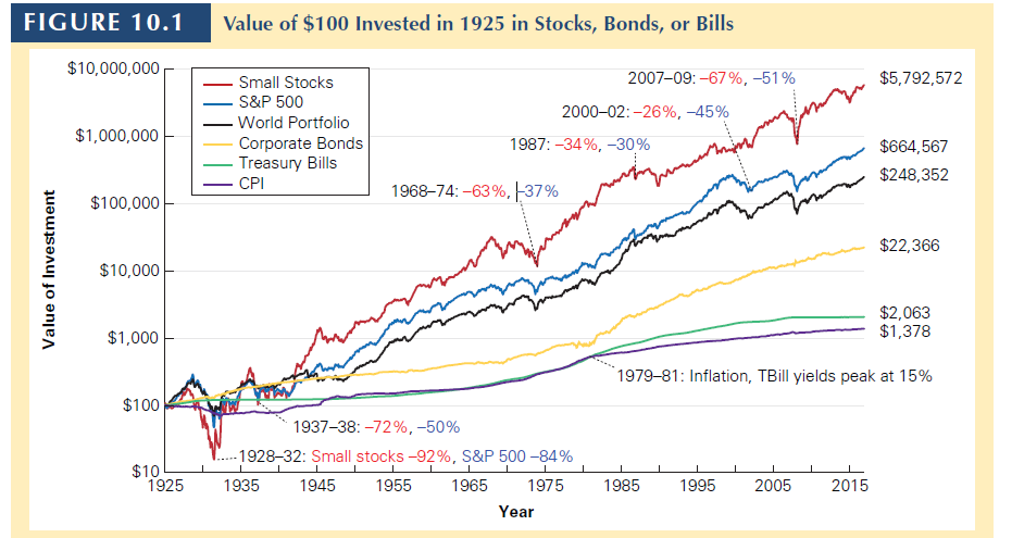
For example, from 1926 to 2017 the average return of the S&P 500 was 12.0% with a volatility of 19.8%.

\[E[R] \pm 2\times SE = 12\% \pm \frac{19.8\%}{\sqrt{92}}= 12\% \pm 4.1\%\] This means that, with 95% confidence interval, the expected return of the S&P 500 during this period ranges from 7.9% and 16.1%.

The longer the period, the more accurate you are. But even with 92 years of data, you are not very accurate to predict the expected return of the SP500.

10.4 Tradeoff risk vs. return

10.4 Tradeoff risk vs. return

Investors are assumed to be risk averse:

• To assume risk, they need extra return for that risk.

• They demand excess return.

Excess returns

• The difference between:

  • 1. the average return for an investment with risk, and
  • 2. the average return for risk-free assets.

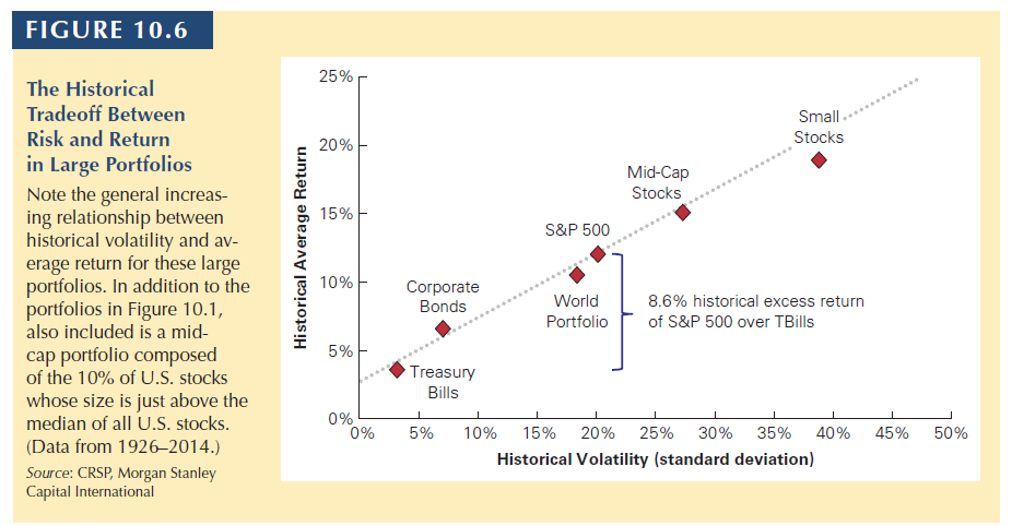
10.4 Tradeoff risk vs. return

That is why riskier assets are expected to have higher returns.

In other words, risk and return have a positive correlation.

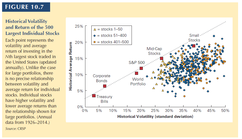
10.4 Tradeoff risk vs. return

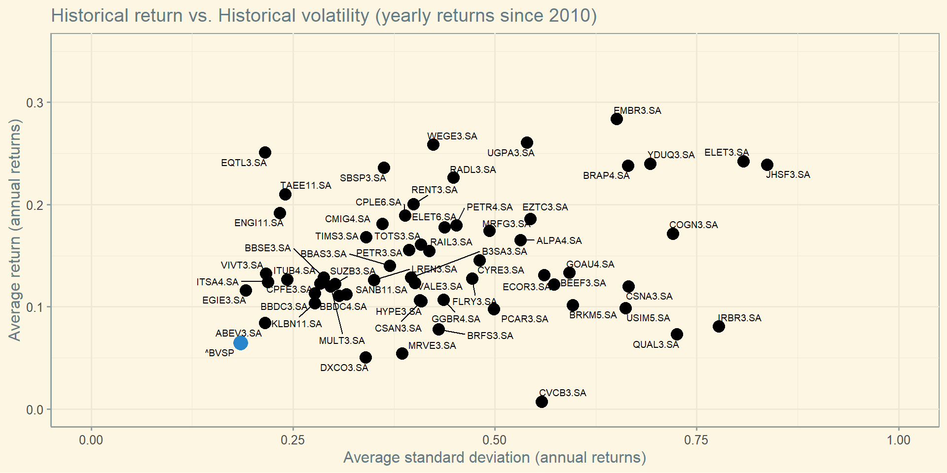
But the association is not linear as one might expect. See stocks below.

Risk vs return of selected Brazilian stocks. There seems to be line, but not really…

start <-'2010-01-01' 
end   <- Sys.Date() 
asset <- yf_collection_get("IBOV", 
                         first_date = start,
                         last_date = end,
                         thresh_bad_data = 0.5,
                         freq_data ="yearly")

Error in dplyr::rename(., ticker = Ticker, company = Company, industry = Industry) : 
  Can't rename columns that don't exist.
✖ Column `Ticker` doesn't exist.

asset<-asset[complete.cases(asset),] 
stocks <-c('^BVSP' ) 
ibov <- yf_get(tickers = stocks, 
                         first_date = start,
                         last_date = end,
                         freq_data ="yearly")
ibov<-ibov[complete.cases(ibov),]
data<-rbind(asset,ibov)
mean_sd  <- data %>%                          
            group_by(ticker) %>%
            summarise_at(vars(ret_adjusted_prices),
                         list(mean = mean,
                              sd = sd)) %>% 
            as.data.frame()
p<-ggplot(mean_sd, aes(x=sd, y=mean)) + 
    ggrepel::geom_text_repel(data = mean_sd, aes(label = ticker) , size = 2.5 ,  max.overlaps = Inf)+
      geom_point(size = 4)  +   xlim(0, 1) + ylim(0, 0.35) + 
        labs(x = "Average standard deviation (annual returns)",
             y='Average return (annual returns)', 
             title="Historical return vs. Historical volatility (yearly returns since 2010)") +   theme_solarized() +
  geom_point(data = mean_sd[mean_sd$ticker == '^BVSP',], color = "#2986cc", size = 5)
p

Key: module2_slide2

Which of the following best describes the risk-return tradeoff in financial markets?

A. Investors are always compensated with higher returns regardless of the risk level.
B. Lower risk assets always outperform higher risk assets in the long run.
C. Assets with higher risk tend to offer higher expected returns as compensation to investors.
D. Risk and return are independent; investors choose based only on preferences.
E. Government bonds have historically delivered the highest returns due to zero risk.

✅ Correct: C. The fundamental principle of the risk-return tradeoff is that investors demand higher expected returns to bear higher risk. Historical data confirm that more volatile asset classes (like small stocks) have yielded higher average returns.

Student ID:

Password:

10.6 Diversification

10.6 Diversification

When you have a portfolio containing assets, the risk you incurred is less than the (weighted average) of the assets’ risk. Let’s understand why.

First, we need to separate two types of risk:

• Firm-specific risk (or news):
  • good or bad news about the company itself. For example, a firm might announce that it has been successful in gaining market share within its industry.
  • this type of risk is independent across firms.
  • also called firm-specific, idiosyncratic, unique, or diversifiable risk.
• Market-wide risk (or news):
  • news about the economy as a whole, affects all stocks. For instance, changes in the interest rates.
  • this type of risk is common to all firms.
  • also called systematic, undiversifiable, or market risk.

10.6 Diversification

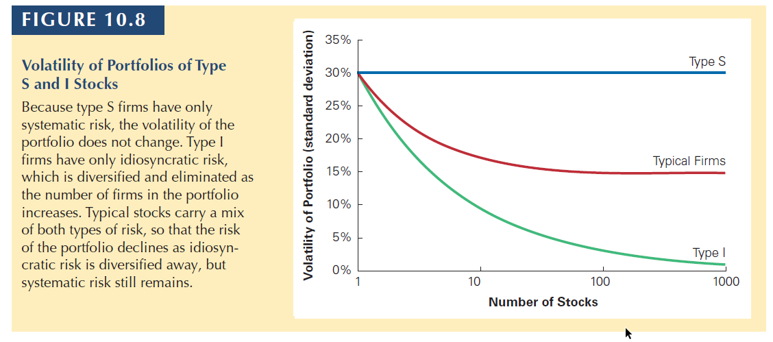
Firm-Specific Versus Systematic Risk

• When many stocks are combined in a large portfolio, the firm-specific risks for each stock will average out and be diversified. The systematic risk, however, will affect all firms and will not be diversified.

Consider two types of firms:

Type S firms are affected only by systematic risk. There is a 50% chance the economy will be strong and they will earn a return of 40%. There is a 50% change the economy will be weak and their return will be −20%. Because all these firms face the same systematic risk, holding a large portfolio of type S firms will not diversify the risk.

Type I firms are affected only by firm-specific risks. Their returns are equally likely to be 35% or −25%, based on factors specific to each firm’s local market. Because these risks are firm specific, if we hold a portfolio of the stocks of many type I firms, the risk is diversified.

10.6 Diversification

You must be aware that actual firms are affected by both market-wide risks and firm-specific risks.

When firms carry both types of risk, only the unsystematic risk will be diversified when many firm’s stocks are combined into a portfolio.

The volatility will therefore decline until only the systematic risk remains.

10.6 Diversification

An additional comment about diversification:

1) it occurs only if the risk of the stocks are independent

• we will define later what “independent” means to us.
• intuitively, different firms have different risks.

2) if the risks are independent, more stocks means less risk…

• … until a certain point.

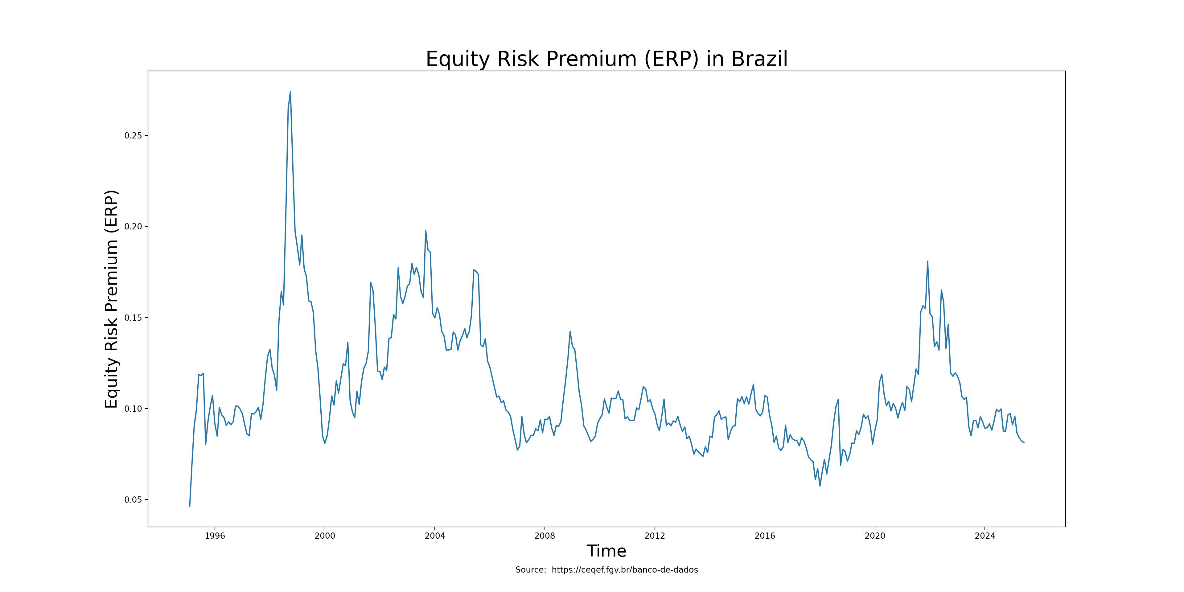
Brazil

United States

10.6 Diversification

Consider again type I firms, which are affected only by firm-specific risk. Because each individual type I firm is risky, should investors expect to earn a risk premium when investing in type I firms?

The risk premium for diversifiable risk is zero, so investors are not compensated for holding firm-specific risk.

• The reason is that they can mitigate this part of risk through diversification.

• Diversification eliminates this risk for free, implying that all investors should have a diversified portfolio. Otherwise, the investor is not rational.

The takeaway is:

The risk premium of a security is determined by its systematic risk and does not depend on its diversifiable risk.

10.6 Diversification

In a world where diversification exists:

Standard deviation is not a good measure for risk anymore.

• Standard deviation is a measure of a stock’s total risk
• But if you are diversified, you are not incurring the total risk, only the systematic risk.

We will need a measure of a stock’s systematic risk.

This measure is called: Beta

But make no mistake:

The standard deviation of the returns of a portfolio is still a good measure for the portfolio’s risk!

• But you will not use the average standard deviation of individual stocks contained in a portfolio.

Key: module2_slide3

How does diversification affect the risk of an investment portfolio?

A. Diversification increases both risk and expected return.
B. Diversification reduces unsystematic (firm-specific) risk but cannot eliminate systematic (market) risk.
C. Diversification guarantees higher returns regardless of market conditions.
D. Diversification eliminates all forms of investment risk.
E. Diversification has no impact on portfolio volatility.

✅ Correct: B. Diversification spreads investments across assets, reducing unsystematic (idiosyncratic) risk tied to individual securities. However, systematic risk — stemming from economy-wide factors — remains even in well-diversified portfolios.

Student ID:

Password:

start <-'2010-01-01' 
end   <- '2025-06-01' 
data <- yf_collection_get("IBOV", 
                         first_date = start,
                         last_date = end,
                         freq_data = "daily",)

Error in dplyr::rename(., ticker = Ticker, company = Company, industry = Industry) : 
  Can't rename columns that don't exist.
✖ Column `Ticker` doesn't exist.

data<-data[complete.cases(data),] 
data$month <- format(as.Date(data$ref_date, format="%y/%m/%d"),"%y/%m")
sd  <-    data %>%                          
            group_by(ticker,month) %>%
            summarise_at(vars(ret_adjusted_prices),list(sd = sd)) %>% 
            as.data.frame()
vol  <-    data %>%                          
            group_by(ticker,month) %>%
            summarise_at(vars(volume),list(vol_sum = sum)) %>% 
            as.data.frame()
vol2  <-    data %>%                          
            group_by(month) %>%
            summarise_at(vars(volume),
                         list(vol_tot = sum)) %>% 
            as.data.frame()
data2 <- merge(sd ,vol, by=c("ticker","month"))
data2 <- merge(data2 ,vol2, by=c("month"))
data2$w <- data2$vol_sum/data2$vol_tot
data2$sdw <- data2$sd * data2$w
data3  <-   data2 %>%                          
            group_by(month) %>%
            summarise_at(vars(sdw),list(total = sum)) %>% 
            as.data.frame()
data3<-data3[complete.cases(data3),] 
data3$id <-"Weighted"
# Index
ibov <- yf_get(tickers = '^BVSP', 
                         first_date = start,
                         last_date = end,
                         freq_data = "daily",)
ibov<-ibov[complete.cases(ibov),] 
ibov$month <- format(as.Date(ibov$ref_date, format="%y/%m/%d"),"%y/%m")
sd2  <-    ibov %>%                          
            group_by(month, ticker) %>%
            summarise_at(vars(ret_closing_prices) ,
                         list(total = var ) ) %>% 
            as.data.frame()
sd2$total <- sd2$total^0.5
sd2$id <-"ibov"
sd2$ticker <- NULL
data4 <- rbind(data3,sd2)
p<-ggplot(data=data4, aes(x=month, y=total, color = id, group = id)) +
  geom_line() + 
        labs(x = "",
             y='Standard deviation',
             title ="Diversification benefits - Ibov vs. Weighted sd of individual stocks") +   theme_solarized()
ggplotly(p)

10.7 Measuring Systematic Risk

10.7 Measuring Systematic Risk

Beta

To measure the systematic risk of a stock, determine how much of the variability of its return is due to systematic risk versus unsystematic risk.

• To determine how sensitive a stock is to systematic risk, look at the average change in the return for each 1% change in the return of a portfolio that fluctuates solely due to systematic risk.

This is the exact definition of a Beta in a regression or a linear relationship (we studied that in statistics).

Saying the same thing in other words:

Beta measures the expected percent change in the excess return of a security for a 1% change in the excess return of the market portfolio.

• Market portfolio contains all stocks: SP500 is a proxy, Ibov is another (for BR).

Market Risk Premium

We can define: The market risk premium is the reward investors expect to earn for holding a portfolio with a beta of 1.

\[Market\; risk\;premium = E[R_m] - R_{rf}\]

Inverting:

\[E[R_m] = R_{rf} + Market\; risk\;premium\]

The idea is that investors are risk-averse and dislike risk. Therefore, in order to invest in risky assets, investors demand an extra return.

Flipping the argument, a risky asset will have to pay an extra return for its additional risk in order to attract investors.

Therefore, there is a clear association between the risk and return of assets.

Again: in a diversified portfolio, investors are diversified so they only worry about beta (not standard deviation).

Equity Risk Premium (ERP)

• R
• Python

url <- "https://ceqef.fgv.br/sites/default/files/2025-07/Serie%20de%20Equity%20Risk%20Premium%20Junho.xlsx"
download(url, dest="../files/epr.xlsx", mode="wb") 
data <- read_excel("../files/epr.xlsx", col_types = c("date","numeric") )
data <- data[2:nrow(data),1:2]
colnames(data) <- c("month", "erp")

p<-ggplot(data, aes(x=month, y = erp)) + geom_line() + theme_solarized()+
  labs(y = "Equity Risk Premium (ERP)", 
       x = "", 
       title = "Equity Risk Premium (ERP) in Brazil" , 
       caption = "Source: https://ceqef.fgv.br/banco-de-dados" )
ggplotly(p)

import pandas as pd
import matplotlib.pyplot as plt
url = "https://ceqef.fgv.br/sites/default/files/2025-07/Serie%20de%20Equity%20Risk%20Premium%20Junho.xlsx"
data = pd.read_excel(url, header=2)
data = data.iloc[:, 0:2]
data.columns = ["month", "erp"]
fig, ax = plt.subplots(figsize=(20, 10))
ax.plot(data["month"], data["erp"])
ax.set_xlabel("Time", fontsize=20)
ax.set_ylabel("Equity Risk Premium (ERP)", fontsize=20)
ax.set_title("Equity Risk Premium (ERP) in Brazil", fontsize=25)
ax.text(0.5, -0.1, "Source:  https://ceqef.fgv.br/banco-de-dados", transform=ax.transAxes, ha="center")
plt.show()

10.8 Beta and cost of capital

10.8 Beta and cost of capital

Consider an investment with a beta = 1.5.

This investment has 50% more risk than the market portfolio.

Every 1% change in the market portfolio leads to a 1.5% percent change in the investment’s price.

Based on these figures, we can compute the expected return for this investment adjusted by the level or risk it provides.

\[E[R] = R_{rf} + \beta \times (E[R_m] - R_{rf})\]

We will discuss more about this equation later, when discussing the CAPM (Capital Asset Pricing Model).

10.8 Beta and cost of capital

Flipping the argument from the previous slides, we can compute the cost of capital for this investment using the same formula:

\[E[R] = R_{rf} + \beta \times (E[R_m] - R_{rf})\]

Assume the economy has a 60% chance that the market return will be 15% next year and a 40% chance the market return will be 5% next year. Assume the risk-free rate is 6%. If a company’s beta is 1.18, what is its expected return next year?

First, compute \(E[R_m]\):

\[E[R_m] = 60\% \times 15\% + 40\% \times 5\% = 11\%\]

Second, compute \(E[R]\):

\[E[R] = 6\% + 1.18 \times (11\% - 6\%) = 11.9\%\]

Now it is your turn…

✅ True / False Questions

🔢 Numeric Questions

📝 Multiple Choice

✍️ Long-form Answers

🙋‍♂️ Any Questions?

Thank You!

Henrique C. Martins

• 🌐 FGV/EAESP
  
• 💼 LinkedIn
  
• 🧠 Google Scholar
  
• 📄 Lattes CV
  
• 🏠 Personal Website