The following are simple examples of how to compute basic statistics using R. We will start importing the data. Let’s use the free dataset iris, available in R.
We have 5 variables: Sepal.Length, Sepal.Width, Petal.Length, Petal.Width e Species. The first four are numeric while the last is a string with three groups: setosa, versicolor, and virginica. The dataset contains 150 observations
Basic stats
Let’s take a look at the first 10 observations in the dataset.
Now, let’s find the means and the medians of the four numeric variables. The most intuitive way is as follows.
mean(iris$Sepal.Length)
[1] 5.843333
mean(iris$Sepal.Width)
[1] 3.057333
mean(iris$Petal.Length)
[1] 3.758
mean(iris$Petal.Width)
[1] 1.199333
median(iris$Sepal.Length)
[1] 5.8
median(iris$Sepal.Width)
[1] 3
median(iris$Petal.Length)
[1] 4.35
median(iris$Petal.Width)
[1] 1.3
Mean and Median
But this is the easiest way.
summary(iris)
  Sepal.Length    Sepal.Width     Petal.Length    Petal.Width
 Min.   :4.300   Min.   :2.000   Min.   :1.000   Min.   :0.100
 1st Qu.:5.100   1st Qu.:2.800   1st Qu.:1.600   1st Qu.:0.300
 Median :5.800   Median :3.000   Median :4.350   Median :1.300
 Mean   :5.843   Mean   :3.057   Mean   :3.758   Mean   :1.199
 3rd Qu.:6.400   3rd Qu.:3.300   3rd Qu.:5.100   3rd Qu.:1.800
 Max.   :7.900   Max.   :4.400   Max.   :6.900   Max.   :2.500
       Species
 setosa    :50
 versicolor:50
 virginica :50
Mean and Median
See that in the code above you also have the number of observations of each species. If you wanted to know how many observations you have in the dataset, you could use the following line. This might be important in the future.
length(iris$Species)
[1] 150
Mean and Median
If you want the same thing by group, do as follows:
by(iris, iris$Species, summary)
iris$Species: setosa
  Sepal.Length    Sepal.Width     Petal.Length    Petal.Width
 Min.   :4.300   Min.   :2.300   Min.   :1.000   Min.   :0.100
 1st Qu.:4.800   1st Qu.:3.200   1st Qu.:1.400   1st Qu.:0.200
 Median :5.000   Median :3.400   Median :1.500   Median :0.200
 Mean   :5.006   Mean   :3.428   Mean   :1.462   Mean   :0.246
 3rd Qu.:5.200   3rd Qu.:3.675   3rd Qu.:1.575   3rd Qu.:0.300
 Max.   :5.800   Max.   :4.400   Max.   :1.900   Max.   :0.600
       Species
 setosa    :50
 versicolor: 0
 virginica : 0


------------------------------------------------------------
iris$Species: versicolor
  Sepal.Length    Sepal.Width     Petal.Length   Petal.Width          Species
 Min.   :4.900   Min.   :2.000   Min.   :3.00   Min.   :1.000   setosa    : 0
 1st Qu.:5.600   1st Qu.:2.525   1st Qu.:4.00   1st Qu.:1.200   versicolor:50
 Median :5.900   Median :2.800   Median :4.35   Median :1.300   virginica : 0
 Mean   :5.936   Mean   :2.770   Mean   :4.26   Mean   :1.326
 3rd Qu.:6.300   3rd Qu.:3.000   3rd Qu.:4.60   3rd Qu.:1.500
 Max.   :7.000   Max.   :3.400   Max.   :5.10   Max.   :1.800
------------------------------------------------------------
iris$Species: virginica
  Sepal.Length    Sepal.Width     Petal.Length    Petal.Width
 Min.   :4.900   Min.   :2.200   Min.   :4.500   Min.   :1.400
 1st Qu.:6.225   1st Qu.:2.800   1st Qu.:5.100   1st Qu.:1.800
 Median :6.500   Median :3.000   Median :5.550   Median :2.000
 Mean   :6.588   Mean   :2.974   Mean   :5.552   Mean   :2.026
 3rd Qu.:6.900   3rd Qu.:3.175   3rd Qu.:5.875   3rd Qu.:2.300
 Max.   :7.900   Max.   :3.800   Max.   :6.900   Max.   :2.500
       Species
 setosa    : 0
 versicolor: 0
 virginica :50
Minimum and maximum
The function summaryalready gives you the minimum and maximum of all variables. But sometimes you need to find only these values. You could use the following lines.
min(iris$Sepal.Length)
[1] 4.3
max(iris$Sepal.Length)
[1] 7.9
You could also find the range of values to find the extreme values of a variable.
range(iris$Sepal.Length)
[1] 4.3 7.9
Minimum and maximum
If you need the distance between the extreme values, you can use:
R
max(iris$Sepal.Length) -min(iris$Sepal.Length)
[1] 3.6
Standard-deviation and Variance
Finally, you can also compute the Standard-deviation and Variance of one variable as follows.
sd(iris$Sepal.Length)
[1] 0.8280661
var(iris$Sepal.Length)
[1] 0.6856935
If you want the standard deviation of all variables:
The following lines will show you a correlation table. First, you need to create a new dataframe with only the numeric variables. This is an extremely important table to your academic paper.
Here is another important table you might use in your paper: the frequency of observations by group.
table(iris$Species)
    setosa versicolor  virginica
        50         50         50
T-test
Let’s create now a t-test of the difference in means. For that, we will use another dataset: mtcars. The data was extracted from the 1974 Motor Trend US magazine, and comprises fuel consumption and 10 aspects of automobile design and performance for 32 automobiles. You can find the description of the variables here.
You will find that there is one variable that is binary: either the cars are automatic (1) or are manual (0).
When you have binary variables, it is always a good idea to test if the means of the variables are different between the two groups of the binary variable.
This is a big thing and you will use a lot in your academic research. In fact, in many articles, the authors explore and compare two groups. So, be ready to create such an analysis.
T-test
First, import the new dataset. Then, repeat the first steps and inspect this dataset (I will not inspect the dataset here, but you should inspect as a way to practice it).
mtcars <- mtcars
T-test
Then, use the binary variable to see if other variables have similar means. The following case compares the average of mpg (miles p/ gas) of automatic vs. manual car.
t.test(mpg ~ am, data=mtcars)
    Welch Two Sample t-test

data:  mpg by am
t = -3.7671, df = 18.332, p-value = 0.001374
alternative hypothesis: true difference in means between group 0 and group 1 is not equal to 0
95 percent confidence interval:
 -11.280194  -3.209684
sample estimates:
mean in group 0 mean in group 1
       17.14737        24.39231
We see that the average in the automatic car is around 17.1 while the average of manual cars is 24.3.
These averages are statistically different, since the t-stat is high (-3.76).
So, we can learn that automatic cars consume more gas than manual cars.
This type of test will be very important in your research.
Dispersion
These measures show how spread out the data are around the mean.
The coefficient of variation (CV) compares variability relative to the mean — useful in finance for comparing volatility across assets.
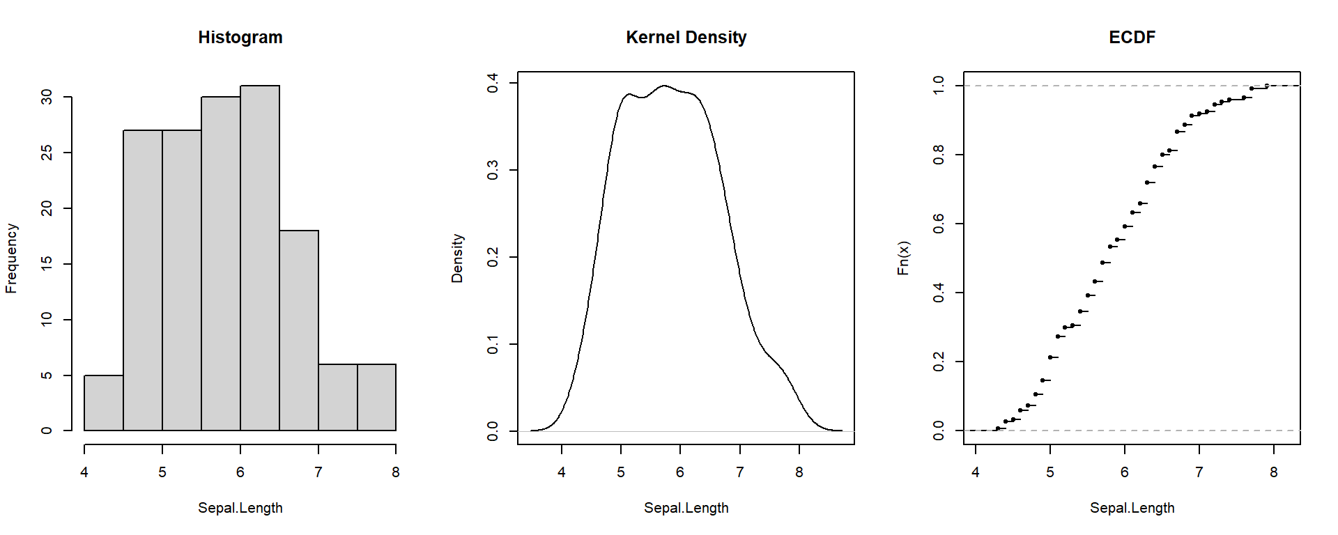
Visualizing the distribution helps you see its shape — whether symmetric, skewed, or concentrated.
Empirical Cumulative Distribution Function (ECDF) = y-axis shows the accumulated proportion of observations below the x-value.
par(mfrow =c(1,3))hist(iris$Sepal.Length, breaks =10, main ="Histogram", xlab ="Sepal.Length")plot(density(iris$Sepal.Length), main ="Kernel Density", xlab ="Sepal.Length")plot(ecdf(iris$Sepal.Length), main ="ECDF", xlab ="Sepal.Length")
par(mfrow =c(1,1))
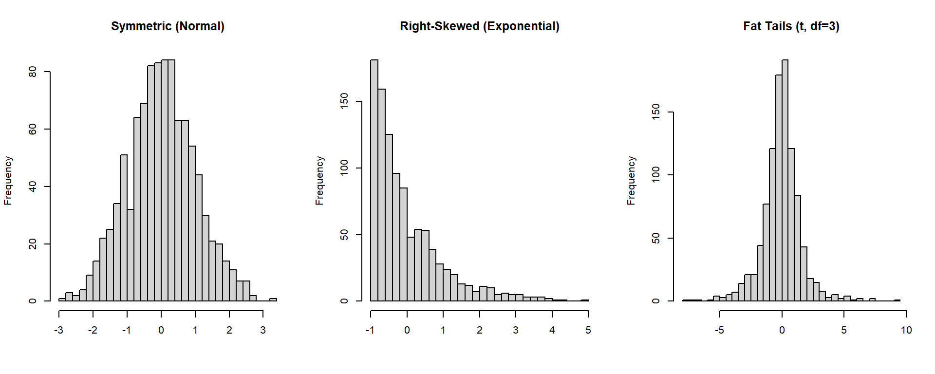
Shape: Skewness & Kurtosis
These measures describe the shape of a distribution.
- Skewness: measures symmetry (right- or left-tailed).
- Kurtosis: measures tail heaviness (fat tails → more extreme events).
set.seed(123)x_sym <-rnorm(1000, mean =0, sd =1) # symmetric (normal)x_right <-rexp(1000, rate =1) -1# right-skewedx_fat <-rt(1000, df =3) # heavy tails (t-distribution)par(mfrow =c(1,3))hist(x_sym, breaks =25, main ="Symmetric (Normal)", col ="lightgray", xlab ="")hist(x_right, breaks =25, main ="Right-Skewed (Exponential)", col ="lightgray", xlab ="")hist(x_fat, breaks =25, main ="Fat Tails (t, df=3)", col ="lightgray", xlab ="")
par(mfrow =c(1,1))
Shape: Skewness & Kurtosis
Now, let’s compute skewness and kurtosis for our actual data.
Skewness > 0 → right tail longer (positive skew).
Skewness < 0 → left tail longer (negative skew).
Kurtosis > 0 → heavier tails than normal (leptokurtic).
Kurtosis < 0 → lighter tails than normal (platykurtic).
skewness <-function(v){ m <-mean(v); s <-sd(v)mean(((v - m)/s)^3)}kurtosis_excess <-function(v){ m <-mean(v); s <-sd(v)mean(((v - m)/s)^4) -3}c(skewness =skewness(iris$Sepal.Length),excess_kurtosis =kurtosis_excess(iris$Sepal.Length))
       skewness excess_kurtosis
      0.3086407      -0.6058125
Outliers via IQR Rule
Outliers are points far from most observations. The IQR rule defines them as values beyond 1.5 × IQR from the quartiles.
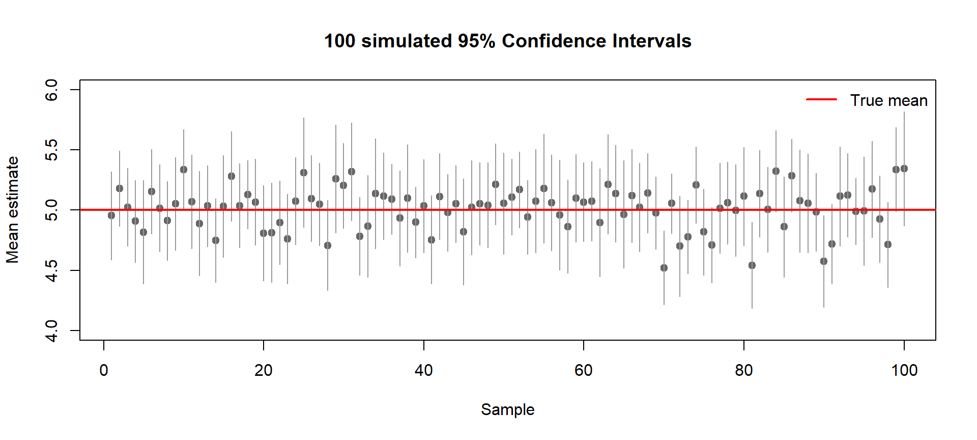
A confidence interval reflects the uncertainty around an estimate.
If we repeat the experiment many times, most intervals will capture the true mean, but some will miss it just by chance.
Below, we simulate 100 random samples (each with 30 observations from a true mean of 5).
Each horizontal line shows a 95% confidence interval for one sample mean.
The red line marks the true mean (μ = 5).
Gray dots: sample means
Gray bars: confidence intervals
Intervals that miss the red line show random sampling error
About 5 out of 100 intervals are expected to miss (≈5%)
👉 A 95% CI means: if we repeated the experiment many times, 95% of the intervals would contain the true mean.
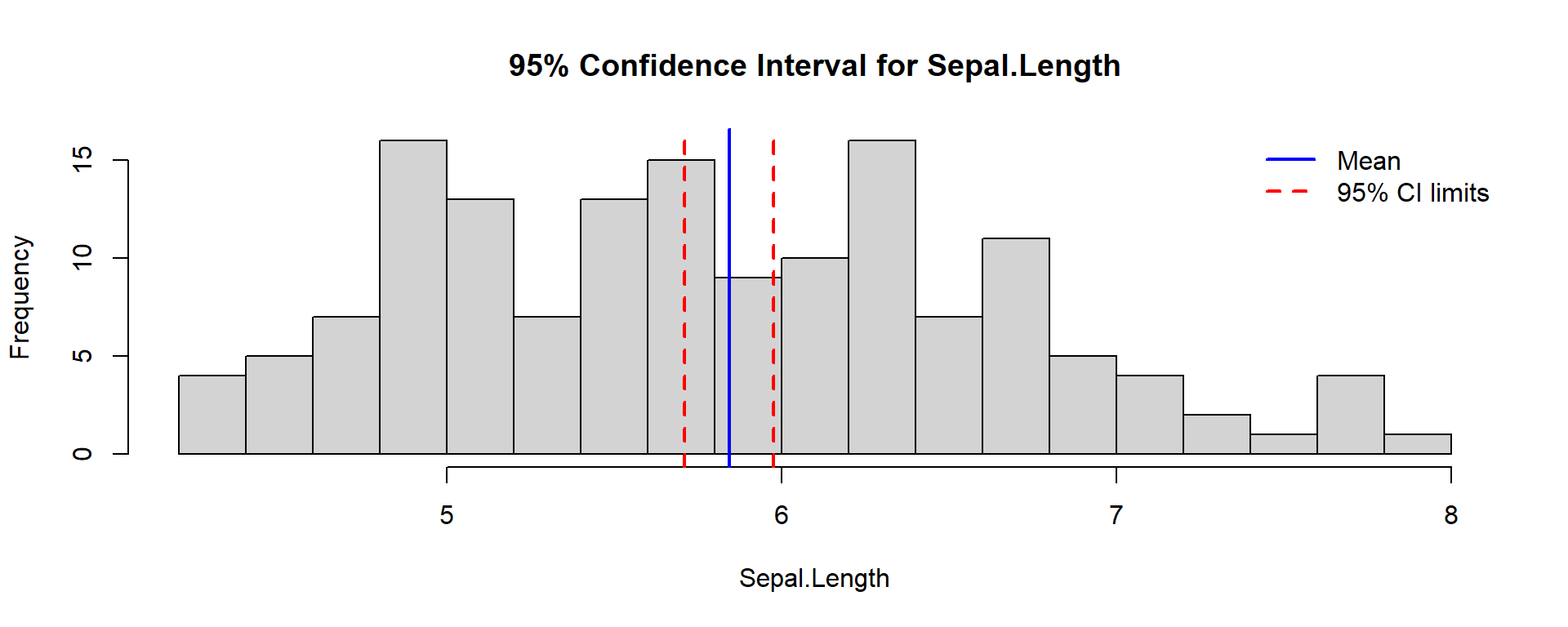
    One Sample t-test

data:  iris$Sepal.Length
t = 86.425, df = 149, p-value < 2.2e-16
alternative hypothesis: true mean is not equal to 0
95 percent confidence interval:
 5.709732 5.976934
sample estimates:
mean of x
 5.843333
👉 The output shows:
Sample mean
Confidence limits
t-statistic and p-value
You can visualize the result below.
x <- iris$Sepal.Lengthm <-mean(x)se <-sd(x)/sqrt(length(x))ci <- m +c(-1,1)*qt(0.975, df=length(x)-1)*sehist(x, breaks =15, col ="lightgray",main ="95% Confidence Interval for Sepal.Length",xlab ="Sepal.Length")abline(v = m, col ="blue", lwd =2)abline(v = ci, col ="red", lty =2, lwd =2)legend("topright", legend=c("Mean", "95% CI limits"), col=c("blue","red"), lwd=2, lty=c(1,2), bty="n")