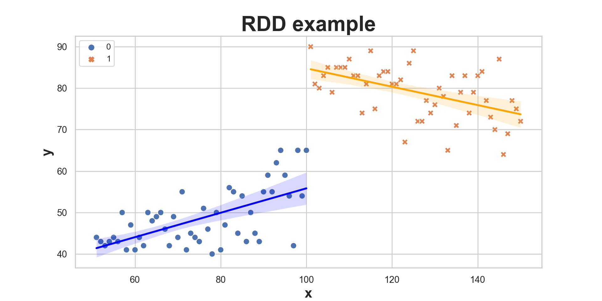
Regression Discontinuity Design (RDD)
Regression Discontinuity Design (RDD)
The regression-discontinuity (RD) research design is a quasi experimental method.
Here the treatment is not a binary as before.
Treated units are assigned based on a cutoff score of a continuous variable.
In a RDD the treatment assignment is not random…
… but it is based in the value of an observed covariate, in which the units lie on either side of the threshold.
Regression Discontinuity Design (RDD)
Example Mastering Metrics:
- Age for drinking is 18 in Brazil.
Why prohibiting younger than 18?
The theory behind this effort is that legal drinking at age 18 discourages binge drinking and promotes a culture of mature alcohol consumption.
The cutoff splits who can drink and who can’t.
Regression Discontinuity Design (RDD)
The name RDD comes from a jump, a discontinuity that occurs in a continuous variable.
In its simplest form, the design has a:
The assignment variable (e.g., age),
Two groups (above and below the cutoff),
The outcome variable.
You may include nonlinearities and control variables.
Regression Discontinuity Design (RDD)
RDD is:
\[D_i = 1(x_i>c) \;\]
where:
\(X\) is called the forcing variable because it “forces” units into treatment or control groups.
\(X\) may be correlated with \(Y_1\) or \(Y_0\), so simply comparing treated and control units would not provide causal effects
However, if the units are randomly assigned into treatment around the cutoff, we would have causal effects.
Regression Discontinuity Design (RDD)
The main assumption that allows using RDD as a causal method is that
Next to the cut, the participants are similar. The only difference is that one individual is in each of the “sides”. Source
![]()
Regression Discontinuity Design (RDD)
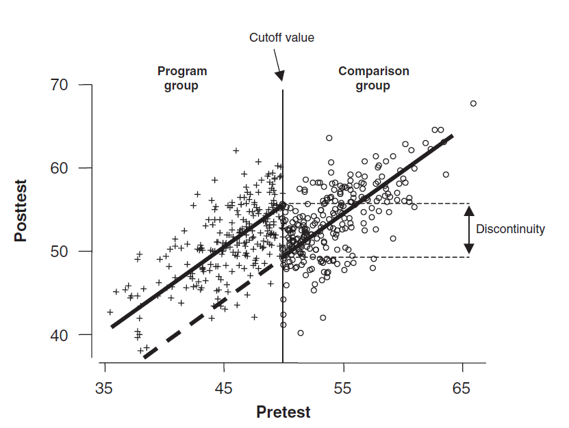
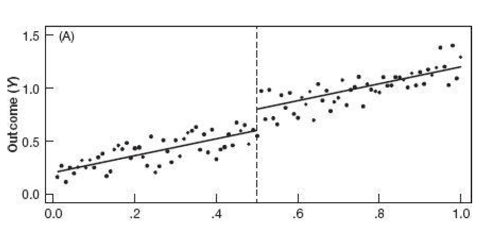
The cutoff value occurs at 50
What are the differences between someone that scores 49.99 and 50.01 in the X variable?
The intuition is that these individuals are similar and comparable.
In the absence of treatment, the assumption is that the solid line would “continue” with the same inclination and values.
There is a discontinuity, however. This implies that the pretreatment in the absence of the treatment should be the dashed line.
The discontinuity is the causal effect of X (at the cutoff) to Y.
Regression Discontinuity Design (RDD)
Unlike the matching and regression strategies based on treatment-control comparisons conditional on covariates, the validity of RDD is based on our willingness to extrapolate across values of the running variable, at least for values in the neighborhood of the cutoff at which treatment switches on. MM
Regression Discontinuity Design (RDD)
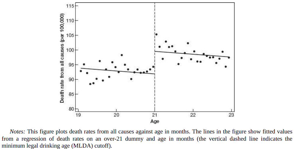
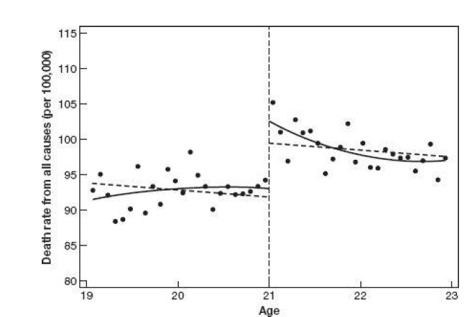
Again the drinking example:
In the US it is 21 years (age & alcohol). Example Mastering Metrics:
Notice the x-axis.
![]()
Regression Discontinuity Design (RDD)
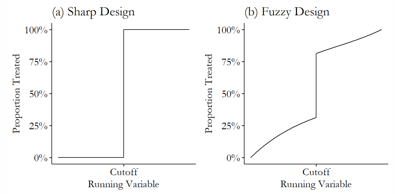
This is (legally, it should be) an example of a Sharp RDD
A Sharp RDD occurs when the cutoff is mandatory. There are no exceptions. In this case, there are no 17 years old drinking and driving.
The treatment is
\[D_a= 1, \;if \;a \;>=\; 18, \;0 \;if \;a\; <\; 18\]
The alternative is a fuzzy RDD, which occurs when there is some misassignment.
- People from under the cut also receiving the treatment.
- Ex. students that receive 5,96 usually are approved in a course (this is a misassignment).
- To estimate a Fuzzy RDD, you can use the treatment as an instrumental variable (Angrist & Pischke, 2009).
Regression Discontinuity Design (RDD)
fuzzy RDD (The effect )
![]()
Regression Discontinuity Design (RDD)
fuzzy RDD
Compliers: Takes treatment if above threshold but not if below threshold.
Always-Takers: Always takes the treatment, ignores the cut.
Never-Takers: Never takes the treatment, ignores the cut.
Defiers: Takes treatment if below the threshold, does not take the treatment if above the threshold.
Regression Discontinuity Design (RDD)
Things that are “good” to a RDD.
- Age
- Dates (you need 6 years to start school, 5,99 years is not allowed)
- Great example: Most of NHL players are those with anniversaries just after the enrollment date
- Ranking systems
- Location (when people cannot “move” easily)
Estimation
A Sharp RDD can take the form of:
\[Y_i = \alpha + \beta_1 D_a + \beta_2 \tilde{x}_1 + \epsilon\]
Where \(D_a\) is the treatment based on the cutoff.
\(x\) is the running variable (the difference between the actual \(X\) and the cutoff in \(X_0\)).
For instance, months until the 18 years birthday.
We can also use the notation: \(\tilde{X}=x-x_0\) regarding the difference.
Estimation
You also should trim the sample to a reasonable window around the cutoff \(c\)
Something like: \(c-h<X_i<c+h\), where \(h\) is a positive value that determines the window
There is no theoretical solution to how big should \(h\) be. It invites robustness tests.
Estimation
Final Step:
Decide on the model of E[Y|X]:
Tip: always execute a visual inspection to check which model os appropriate.
Also, always estimate different models and discuss the results.
Estimation
fuzzy RDD
\[Y_i = \alpha + \beta_1 D_a + \beta_2 \tilde{x}_1 + \beta_3(Z \times \tilde{x}_1) \epsilon\]
Where Z is 1 if unit is above the cut or 0 if unit is below the cut.
Notice that D is not equal to Z, in these cases.
RDD Nonlinearities
Example Mastering Metrics:
This is a linear relationship, with the same slopes.
![]()
\[E[Y|X,D] = \alpha + \beta_1 \times D + \beta_2 \times \tilde{X}\]
RDD Nonlinearities
The effect This is a linear relationship, with different slopes.
![]()
RDD Nonlinearities
Example Mastering Metrics:
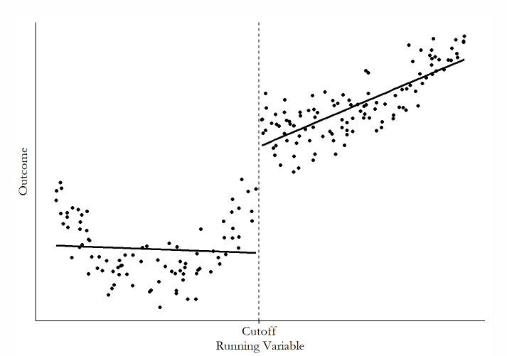
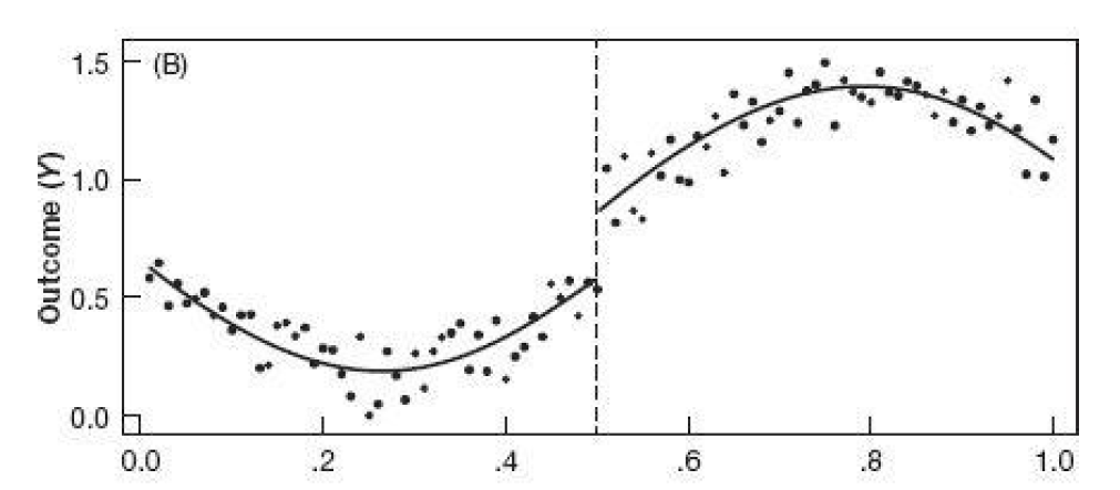
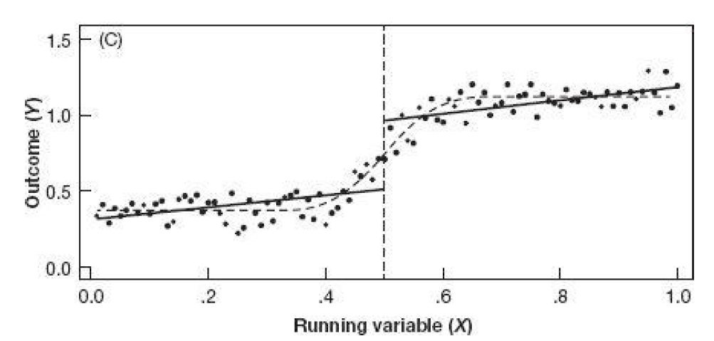
Is the relationship linear or nonlinear here? If you misjudge the relationship, it will be hard to tell a story credibly.
![]()
RDD Nonlinearities
The takeaway: RDD is a graphical method. You need to show the graphs.
Nobody will believe your story without the correct specification of the model.
In the first case:
\[Y_i = \alpha + \beta_1 D_a + \beta_2 x_1 + \epsilon\]
In the second case:
\[Y_i = \alpha + \beta_1 D_a + \beta_2 x_1 + \beta_3 x_1^2 + \epsilon\]
RDD Nonlinearities
We can also add an interaction term (notice that I am changing the notation now to make it similar to MM)
\[Y_i = \alpha + \beta_1 D_a + \beta_2 (x - x_0) + \beta_3 (x - x_0) D_a + \epsilon\]
This allows for different inclinations before and after the cut.
RDD Nonlinearities
Or even different nonlinearities before and after the cut:
\[Y_i = \alpha + \beta_1 D_a + \beta_2 (x - x_0) + \beta_3 (x - x_0)^2 + \beta_4 (x - x_0) D_a + \beta_5 (x - x_0)^2 D_a + \epsilon\]
![]()
