Empirical Methods in Finance

Part 3

Henrique C. Martins

Conterfactuals

Conterfactuals

  • Imagine that John and Mary are moving to the north of Canada.

  • John has a history of respiratory disease and decide to buy insurance.

  • Mary does not have a history of respiratory disease and decide not to buy insurance.

  • What is the causal effect of buying insurance?

Default John Mary
State of insurance 1 0
Situation without insurance n.o. 5
Situation with insurance 4 n.o.
Observed 4 5
Effect ? ?

Source: Mastering Metrics

Conterfactuals

Naïve calculation: comparing John com Mary

\[Y_{john} - Y_{Mary} = 4 - 5 = -1\]

Conclusion: buying insurance has a negative effect on health.

This is wrong!

Source: Mastering Metrics

Conterfactuals

Default John Mary
State of insurance 1 0
Situation without insurance 3 5
Situation with insurance 4 5
Observed 4 5
Effect ? ?

\[(Y_{1,john} - Y_{0,john}) + (Y_{1,Mary}- Y_{0,Mary}) = 4 - 3 + 5 - 5 = 0.5\]

Conclusion: buying insurance has a positive effect of 1 in John’s health and average effect of 0.5 in the sample’s health (i.e. averages conditional on insurance status).

Source: Mastering Metrics

Regressions

Regression Source: Mastering Metrics

Let’s see how a regression could solve the problem. Imagine that you have the following data on students’ application. (Decisions in bold)

Student Private Private Private Public Public Public Earnings
Ivy Leafy Smart State Tall Altered 110,000
1 Reject Admit Admit 110,000
2 Reject Admit Admit 100,000
3 Reject Admit Admit 110,000
4 Admit Admit Admit Admit 60,000
5 Admit Admit Admit Admit 30,000
6 Admit 115,000
7 Admit 75,000
8 Reject Admit Admit 90,000
9 Reject Admit Admit 60,000

Regression Source: Mastering Metrics

We can see from the table that:

  • Some students earn high salary, in both situations

  • Some students earn low salary, in both situations

  • There are clusters of students that applied for the same universities

    • How likely are they to be similar? Can we benefit from the fact they believe they are similar?
  • If we compare earnings from the first three individuals:

    • ((110 + 100)/ 2 - 11000) = -5.000
  • If we compare earnings from individuals 4 and 5:

    • (60 - 30) = 30.000
  • The average is:

    • 25.000/2 = 12.500

Regression Source

Let’s create a dataframe to run regressions with the previous student’s data.

R
# Create the data frame
data <- data.frame(
  id = 1:9,
  earnings = c(110000, 100000, 110000, 60000, 30000, 115000, 75000, 90000, 60000),
  school = c("private", "private", "public", "private", "public", "private", "private", "public", "public"),
  private = c(1, 1, 0, 1, 0, 1, 1, 0, 0),
  group = c(1, 1, 1, 2, 2, 3, 3, 4, 4)
)
print(data)
  id earnings  school private group
1  1   110000 private       1     1
2  2   100000 private       1     1
3  3   110000  public       0     1
4  4    60000 private       1     2
5  5    30000  public       0     2
6  6   115000 private       1     3
7  7    75000 private       1     3
8  8    90000  public       0     4
9  9    60000  public       0     4
Python
import pandas as pd
data = pd.DataFrame({
    'id': range(1, 10),
    'earnings': [110000, 100000, 110000, 60000, 30000, 115000, 75000, 90000, 60000],
    'school': ["private", "private", "public", "private", "public", "private", "private", "public", "public"],
    'private': [1, 1, 0, 1, 0, 1, 1, 0, 0],
    'group': [1, 1, 1, 2, 2, 3, 3, 4, 4]
})
print(data)
   id  earnings   school  private  group
0   1    110000  private        1      1
1   2    100000  private        1      1
2   3    110000   public        0      1
3   4     60000  private        1      2
4   5     30000   public        0      2
5   6    115000  private        1      3
6   7     75000  private        1      3
7   8     90000   public        0      4
8   9     60000   public        0      4
Stata
input id earnings str7 school private group
1 110000 "private" 1 1
2 100000 "private" 1 1
3 110000 "public" 0 1
4 60000 "private" 1 2
5 30000 "public" 0 2
6 115000 "private" 1 3
7 75000 "private" 1 3
8 90000 "public" 0 4
9 60000 "public" 0 4
end
list
            id   earnings     school    private      group
  1. 1 110000 "private" 1 1
  2. 2 100000 "private" 1 1
  3. 3 110000 "public" 0 1
  4. 4 60000 "private" 1 2
  5. 5 30000 "public" 0 2
  6. 6 115000 "private" 1 3
  7. 7 75000 "private" 1 3
  8. 8 90000 "public" 0 4
  9. 9 60000 "public" 0 4
 10. end

     +-------------------------------------------+
     | id   earnings    school   private   group |
     |-------------------------------------------|
  1. |  1     110000   private         1       1 |
  2. |  2     100000   private         1       1 |
  3. |  3     110000    public         0       1 |
  4. |  4      60000   private         1       2 |
  5. |  5      30000    public         0       2 |
     |-------------------------------------------|
  6. |  6     115000   private         1       3 |
  7. |  7      75000   private         1       3 |
  8. |  8      90000    public         0       4 |
  9. |  9      60000    public         0       4 |
     +-------------------------------------------+

“Naive” regression all students Source

\[earnings_i = \alpha + \beta_1 Private_i + \epsilon\] What is the benefit of private education here?

R
# Create the data frame
model <- lm(earnings ~ private, data = data)
summary(model)

Call:
lm(formula = earnings ~ private, data = data)

Residuals:
   Min     1Q Median     3Q    Max 
-42500 -17000   8000  18000  37500 

Coefficients:
            Estimate Std. Error t value Pr(>|t|)   
(Intercept)    72500      14522   4.992  0.00158 **
private        19500      19484   1.001  0.35023   
---
Signif. codes:  0 '***' 0.001 '**' 0.01 '*' 0.05 '.' 0.1 ' ' 1

Residual standard error: 29040 on 7 degrees of freedom
Multiple R-squared:  0.1252,    Adjusted R-squared:  0.0002116 
F-statistic: 1.002 on 1 and 7 DF,  p-value: 0.3502
Python
#pip install numpy scikit-learn statsmodels
import statsmodels.api as sm
X = sm.add_constant(data['private'])  
y = data['earnings']
model = sm.OLS(y, X).fit()
print(model.summary())
                            OLS Regression Results                            
==============================================================================
Dep. Variable:               earnings   R-squared:                       0.125
Model:                            OLS   Adj. R-squared:                  0.000
Method:                 Least Squares   F-statistic:                     1.002
Date:                qua, 11 set 2024   Prob (F-statistic):              0.350
Time:                        16:33:20   Log-Likelihood:                -104.13
No. Observations:                   9   AIC:                             212.3
Df Residuals:                       7   BIC:                             212.7
Df Model:                           1                                         
Covariance Type:            nonrobust                                         
==============================================================================
                 coef    std err          t      P>|t|      [0.025      0.975]
------------------------------------------------------------------------------
const        7.25e+04   1.45e+04      4.992      0.002    3.82e+04    1.07e+05
private      1.95e+04   1.95e+04      1.001      0.350   -2.66e+04    6.56e+04
==============================================================================
Omnibus:                        1.011   Durbin-Watson:                   2.352
Prob(Omnibus):                  0.603   Jarque-Bera (JB):                0.666
Skew:                          -0.263   Prob(JB):                        0.717
Kurtosis:                       1.776   Cond. No.                         2.77
==============================================================================

Notes:
[1] Standard Errors assume that the covariance matrix of the errors is correctly specified.
Stata
quiet input id earnings str7 school private group
1 110000 "private" 1 1
2 100000 "private" 1 1
3 110000 "public" 0 1
4 60000 "private" 1 2
5 30000 "public" 0 2
6 115000 "private" 1 3
7 75000 "private" 1 3
8 90000 "public" 0 4
9 60000 "public" 0 4
end

reg earnings private 
      Source |       SS           df       MS      Number of obs   =         9
-------------+----------------------------------   F(1, 7)         =      1.00
       Model |   845000000         1   845000000   Prob > F        =    0.3502
    Residual |  5.9050e+09         7   843571429   R-squared       =    0.1252
-------------+----------------------------------   Adj R-squared   =    0.0002
       Total |  6.7500e+09         8   843750000   Root MSE        =     29044

------------------------------------------------------------------------------
    earnings | Coefficient  Std. err.      t    P>|t|     [95% conf. interval]
-------------+----------------------------------------------------------------
     private |      19500   19483.51     1.00   0.350    -26571.18    65571.18
       _cons |      72500   14522.15     4.99   0.002     38160.57    106839.4
------------------------------------------------------------------------------

“Naive” regression all students Source

\[earnings_i = \alpha + \beta_1 Private_i + \epsilon\] What is the benefit of private education here?

The coefficient of private is 19500, meaning that those that have private education earn 19500 more.

The problem with this design is that 1) we are including all students, even those that do not bring any “information”, and 2) we are not controlling for the differences in students’ profiles.

Let’s fix the first problem first.

What students should we not include in the model?

Students id<=5 Source

\[earnings_i = \alpha + \beta_1 Private_i + \epsilon \;,\; if\; i <=5\] What is the benefit of private education here?

R
model2 <- lm(earnings ~ private , data = subset(data,id<=5))
summary(model2)

Call:
lm(formula = earnings ~ private, data = subset(data, id <= 5))

Residuals:
     1      2      3      4      5 
 20000  10000  40000 -30000 -40000 

Coefficients:
            Estimate Std. Error t value Pr(>|t|)  
(Intercept)    70000      27689   2.528   0.0856 .
private        20000      35746   0.560   0.6149  
---
Signif. codes:  0 '***' 0.001 '**' 0.01 '*' 0.05 '.' 0.1 ' ' 1

Residual standard error: 39160 on 3 degrees of freedom
Multiple R-squared:  0.09449,   Adjusted R-squared:  -0.2073 
F-statistic: 0.313 on 1 and 3 DF,  p-value: 0.6149
Python
#pip install numpy scikit-learn statsmodels

subset_data = data[data['id'] <= 5]
X = sm.add_constant(subset_data['private']) 
y = subset_data['earnings']
model2 = sm.OLS(y, X).fit()
print(model2.summary())
                            OLS Regression Results                            
==============================================================================
Dep. Variable:               earnings   R-squared:                       0.094
Model:                            OLS   Adj. R-squared:                 -0.207
Method:                 Least Squares   F-statistic:                    0.3130
Date:                qua, 11 set 2024   Prob (F-statistic):              0.615
Time:                        16:33:23   Log-Likelihood:                -58.694
No. Observations:                   5   AIC:                             121.4
Df Residuals:                       3   BIC:                             120.6
Df Model:                           1                                         
Covariance Type:            nonrobust                                         
==============================================================================
                 coef    std err          t      P>|t|      [0.025      0.975]
------------------------------------------------------------------------------
const           7e+04   2.77e+04      2.528      0.086   -1.81e+04    1.58e+05
private         2e+04   3.57e+04      0.560      0.615   -9.38e+04    1.34e+05
==============================================================================
Omnibus:                          nan   Durbin-Watson:                   1.304
Prob(Omnibus):                    nan   Jarque-Bera (JB):                0.520
Skew:                          -0.129   Prob(JB):                        0.771
Kurtosis:                       1.441   Cond. No.                         2.92
==============================================================================

Notes:
[1] Standard Errors assume that the covariance matrix of the errors is correctly specified.
Stata
quiet input id earnings str7 school private group
1 110000 "private" 1 1
2 100000 "private" 1 1
3 110000 "public" 0 1
4 60000 "private" 1 2
5 30000 "public" 0 2
6 115000 "private" 1 3
7 75000 "private" 1 3
8 90000 "public" 0 4
9 60000 "public" 0 4
end
reg earnings private if id<=5
      Source |       SS           df       MS      Number of obs   =         5
-------------+----------------------------------   F(1, 3)         =      0.31
       Model |   480000000         1   480000000   Prob > F        =    0.6149
    Residual |  4.6000e+09         3  1.5333e+09   R-squared       =    0.0945
-------------+----------------------------------   Adj R-squared   =   -0.2073
       Total |  5.0800e+09         4  1.2700e+09   Root MSE        =     39158

------------------------------------------------------------------------------
    earnings | Coefficient  Std. err.      t    P>|t|     [95% conf. interval]
-------------+----------------------------------------------------------------
     private |      20000   35746.02     0.56   0.615    -93759.78    133759.8
       _cons |      70000   27688.75     2.53   0.086    -18117.95    158117.9
------------------------------------------------------------------------------

Students id<=5 Source

\[earnings_i = \alpha + \beta_1 Private_i + \epsilon \;,\; if\; i <=5\] What is the benefit of private education here?

Students 6 and 7 only applied to Private, while students 8 and 9 did not really had a choice. So we should exclude them.

The benefit of private is now 20000.

The coefficient did not change much, but the design improved partially.

We still have an uncontrolled “heterogeneity” in the groups of students. Students 1 to 3 seem to earn more no matter their decisions.

Apples-to-Apples Source

\[earnings_i = \alpha + \beta_1 Private_i + \beta_2 Group+ \epsilon \;,\; if\; i <=5\] This is the best we can do.

R
data$dummy <- ifelse(data$group == 1, 1, 0)
data$dummy[data$group == 2] <- 0
model3 <- lm(earnings ~ private + dummy, data = subset(data,id<=5))
summary(model3)

Call:
lm(formula = earnings ~ private + dummy, data = subset(data, 
    id <= 5))

Residuals:
         1          2          3          4          5 
 1.182e-11 -1.000e+04  1.000e+04  1.000e+04 -1.000e+04 

Coefficients:
            Estimate Std. Error t value Pr(>|t|)  
(Intercept)    40000      11952   3.347   0.0789 .
private        10000      13093   0.764   0.5248  
dummy          60000      13093   4.583   0.0445 *
---
Signif. codes:  0 '***' 0.001 '**' 0.01 '*' 0.05 '.' 0.1 ' ' 1

Residual standard error: 14140 on 2 degrees of freedom
Multiple R-squared:  0.9213,    Adjusted R-squared:  0.8425 
F-statistic:  11.7 on 2 and 2 DF,  p-value: 0.07874
Python
#pip install numpy scikit-learn statsmodels

data['dummy'] = 1
data.loc[data['group'] == 2, 'dummy'] = 0
subset_data = data[data['id'] <= 5]
X = sm.add_constant(subset_data[['private', 'dummy']])
y = subset_data['earnings']
model3 = sm.OLS(y, X).fit()
print(model3.summary())
                            OLS Regression Results                            
==============================================================================
Dep. Variable:               earnings   R-squared:                       0.921
Model:                            OLS   Adj. R-squared:                  0.843
Method:                 Least Squares   F-statistic:                     11.70
Date:                qua, 11 set 2024   Prob (F-statistic):             0.0787
Time:                        16:33:25   Log-Likelihood:                -52.589
No. Observations:                   5   AIC:                             111.2
Df Residuals:                       2   BIC:                             110.0
Df Model:                           2                                         
Covariance Type:            nonrobust                                         
==============================================================================
                 coef    std err          t      P>|t|      [0.025      0.975]
------------------------------------------------------------------------------
const           4e+04    1.2e+04      3.347      0.079   -1.14e+04    9.14e+04
private         1e+04   1.31e+04      0.764      0.525   -4.63e+04    6.63e+04
dummy           6e+04   1.31e+04      4.583      0.044    3665.052    1.16e+05
==============================================================================
Omnibus:                          nan   Durbin-Watson:                   2.250
Prob(Omnibus):                    nan   Jarque-Bera (JB):                0.638
Skew:                           0.000   Prob(JB):                        0.727
Kurtosis:                       1.250   Cond. No.                         3.49
==============================================================================

Notes:
[1] Standard Errors assume that the covariance matrix of the errors is correctly specified.
Stata
quiet input id earnings str7 school private group
1 110000 "private" 1 1
2 100000 "private" 1 1
3 110000 "public" 0 1
4 60000 "private" 1 2
5 30000 "public" 0 2
6 115000 "private" 1 3
7 75000 "private" 1 3
8 90000 "public" 0 4
9 60000 "public" 0 4
end
gen     dummy = 1 if group == 1
replace dummy = 0 if group == 2
reg earnings private dummy if id<=5 
(6 missing values generated)

(2 real changes made)

      Source |       SS           df       MS      Number of obs   =         5
-------------+----------------------------------   F(2, 2)         =     11.70
       Model |  4.6800e+09         2  2.3400e+09   Prob > F        =    0.0787
    Residual |   400000000         2   200000000   R-squared       =    0.9213
-------------+----------------------------------   Adj R-squared   =    0.8425
       Total |  5.0800e+09         4  1.2700e+09   Root MSE        =     14142

------------------------------------------------------------------------------
    earnings | Coefficient  Std. err.      t    P>|t|     [95% conf. interval]
-------------+----------------------------------------------------------------
     private |      10000   13093.07     0.76   0.525    -46334.95    66334.95
       dummy |      60000   13093.07     4.58   0.044     3665.052    116334.9
       _cons |      40000   11952.29     3.35   0.079    -11426.54    91426.54
------------------------------------------------------------------------------

Regression

The previous regression assumes that students 1 to 3 are different that students 4 and 5.

We will find many instances like that in empirical research. E.g., industry.

The private school coefficient, in this case 10,000, implies a private-public earnings differential of this value.

Important

The Y above is used in monetary values.

Using a logged y, ln(Y) or ln(earnings), allows estimates to be interpreted as a percent change.

For instance if \(\beta=0.05\), it means that the earnings differential is 5% for those studying in private schools (conditional on the controls included in the model).

OVB again

OVB again

Regression is a way to make other things equal (ceteris paribus), but equality is generated only for variables included in the model as controls on the right-hand sided of the model.

Failure to include enough controls of the right controls still leave us with selection bias.

The regression version of the selection bias generated by the inadequate controls is called Omitted Variable Bias (OVB).

The inclusion of a control that should not be included is called “Bad Controls” problem.

OVB again

How could we calculate the OVB in this example?

\[earnings_i = 70.000 + 20.000\times Private_i \epsilon \]

\[earnings_i = 40.000 + 10.000 \times Private_i + 60.000 \times Group+ \epsilon\]

  • \(\beta\) (1st regression) - \(\beta\) (second regression).
  • The OVB here is 20.000 - 10.000 = 10.000.
  • Meaning that the \(\beta\) (1st regression) is 10.000 higher than what it should be.

OVB again

How could we calculate the OVB in this example?

We could calculate the bias by estimating:

\[Private=\alpha + \beta_{omitted} \times Group + \epsilon\]

Then,

\[\beta_{omitted} \times \beta_{missing} = 0.1667 * 60.000 = 10.000\]

The OVB is 10.000, meaning that the first model (the one with the omitted variable) estimates a Beta that is 10.000 higher than it should be.

OVB again

R
model4 <- lm(private ~ dummy , data = subset(data,id<=5))
summary(model4)

Call:
lm(formula = private ~ dummy, data = subset(data, id <= 5))

Residuals:
      1       2       3       4       5 
 0.3333  0.3333 -0.6667  0.5000 -0.5000 

Coefficients:
            Estimate Std. Error t value Pr(>|t|)
(Intercept)   0.5000     0.4410   1.134    0.339
dummy         0.1667     0.5693   0.293    0.789

Residual standard error: 0.6236 on 3 degrees of freedom
Multiple R-squared:  0.02778,   Adjusted R-squared:  -0.2963 
F-statistic: 0.08571 on 1 and 3 DF,  p-value: 0.7888
R
matrix2<- summary(model4)$coefficients
sum(0.1667 * 60000 )
[1] 10002
Python
subset_data = data[data['id'] <= 5]
model4 = sm.OLS(subset_data['private'], sm.add_constant(subset_data[['dummy']])).fit()
print(model4.summary())
                            OLS Regression Results                            
==============================================================================
Dep. Variable:                private   R-squared:                       0.028
Model:                            OLS   Adj. R-squared:                 -0.296
Method:                 Least Squares   F-statistic:                   0.08571
Date:                qua, 11 set 2024   Prob (F-statistic):              0.789
Time:                        16:33:28   Log-Likelihood:                -3.4565
No. Observations:                   5   AIC:                             10.91
Df Residuals:                       3   BIC:                             10.13
Df Model:                           1                                         
Covariance Type:            nonrobust                                         
==============================================================================
                 coef    std err          t      P>|t|      [0.025      0.975]
------------------------------------------------------------------------------
const          0.5000      0.441      1.134      0.339      -0.903       1.903
dummy          0.1667      0.569      0.293      0.789      -1.645       1.978
==============================================================================
Omnibus:                          nan   Durbin-Watson:                   2.881
Prob(Omnibus):                    nan   Jarque-Bera (JB):                0.749
Skew:                          -0.394   Prob(JB):                        0.688
Kurtosis:                       1.276   Cond. No.                         2.92
==============================================================================

Notes:
[1] Standard Errors assume that the covariance matrix of the errors is correctly specified.
Python
bias = 0.1667 * 60000
print(bias)
10002.0
Stata
quiet input id earnings str7 school private group
1 110000 "private" 1 1
2 100000 "private" 1 1
3 110000 "public" 0 1
4 60000 "private" 1 2
5 30000 "public" 0 2
6 115000 "private" 1 3
7 75000 "private" 1 3
8 90000 "public" 0 4
9 60000 "public" 0 4
end
gen     dummy = 1 if group == 1
replace dummy = 0 if group == 2
reg private dummy if id<=5
di .1666667 *  60000 
(6 missing values generated)

(2 real changes made)

      Source |       SS           df       MS      Number of obs   =         5
-------------+----------------------------------   F(1, 3)         =      0.09
       Model |  .033333333         1  .033333333   Prob > F        =    0.7888
    Residual |  1.16666667         3  .388888889   R-squared       =    0.0278
-------------+----------------------------------   Adj R-squared   =   -0.2963
       Total |         1.2         4          .3   Root MSE        =    .62361

------------------------------------------------------------------------------
     private | Coefficient  Std. err.      t    P>|t|     [95% conf. interval]
-------------+----------------------------------------------------------------
       dummy |   .1666667    .569275     0.29   0.789    -1.645021    1.978354
       _cons |         .5   .4409586     1.13   0.339    -.9033269    1.903327
------------------------------------------------------------------------------

10000.002

OVB again

So what?

  • Anticipating the effect of the omitted variable on the non-omitted variable can tell you the sign of the bias.

  • Then you can know if the bias is attenuating or increasing the effect you are investigating.

  • If attenuating, the problem is smaller than if it is increasing

OVB again

Regressions

  • The previous examples show that we can run regressions and find correlations

  • … And we can run regressions and find causal effects.

  • But we need to control for all relevant variables, otherwise we have the OVB problem.

  • Should you not look careful to your data, you’d miss the inclusion of the variable group.

  • The results show that you may estimate a spurious coefficient twice the size of the “true” coefficient.

Bad Controls Problem

Bad Controls Problem

Bad controls are variables that are also outcome of the treatment being studied.

A Bad control could very well be a dependent variable of the treatment as well.

Good controls are variables that you can think as being fixed at the time of the treatment.

Let’s return to the model.

\[earnings_i = \alpha + \beta_1 Private_i + \beta_2 Group+ \epsilon \;,\; if\; i <=5\]

Assuming you also have the occupation of the students at the time of earnings. Should you include occupation in the model?

\[earnings_i = \alpha + \beta_1 Private_i + \beta_2 Group + \beta_3 Occupation + \epsilon \;,\; if\; i <=5\]

Reasoning: “We should use occupation as control because it would be wise to look at the effect of education on earnings only for those within an occupation”.

What is the problem with this reasoning?

Bad Controls Problem

The problem is that studying in private would increase the chances of getting a white-collar occupation, i.e., private education (treatment) affects the occupation (bad control).

In this case, should you include occupation as control, the coefficient of interest no longer has a causal interpretation.

This is a very common problem in empirical research.

It is not hard to come up with stories of why a control is a bad control.

Randomization

Randomization

Now I want to discuss the idea of randomization

Suppose you have developed a treatment (e.g., a program) that you believe will increase the ‘motivation’ of employees of a factory.

You have 100 employees to use in an experiment to test your claim that the treatment will increase motivation.

  • You randomly allocate 50 employees to receive the treatment. The other 50 are part of the control group.
  • You treat all employees in the same manner, except for the treatment.

Using the data available, this is the difference in motivation between the treatment and control groups (next slide):

Randomization

R
library(readxl)
library(ggplot2)
library(tidyverse)
library(dplyr)
data  <- read_excel("files/part_3_data.xlsx", range = "A1:C101")
# Box plot control vs treatment groups
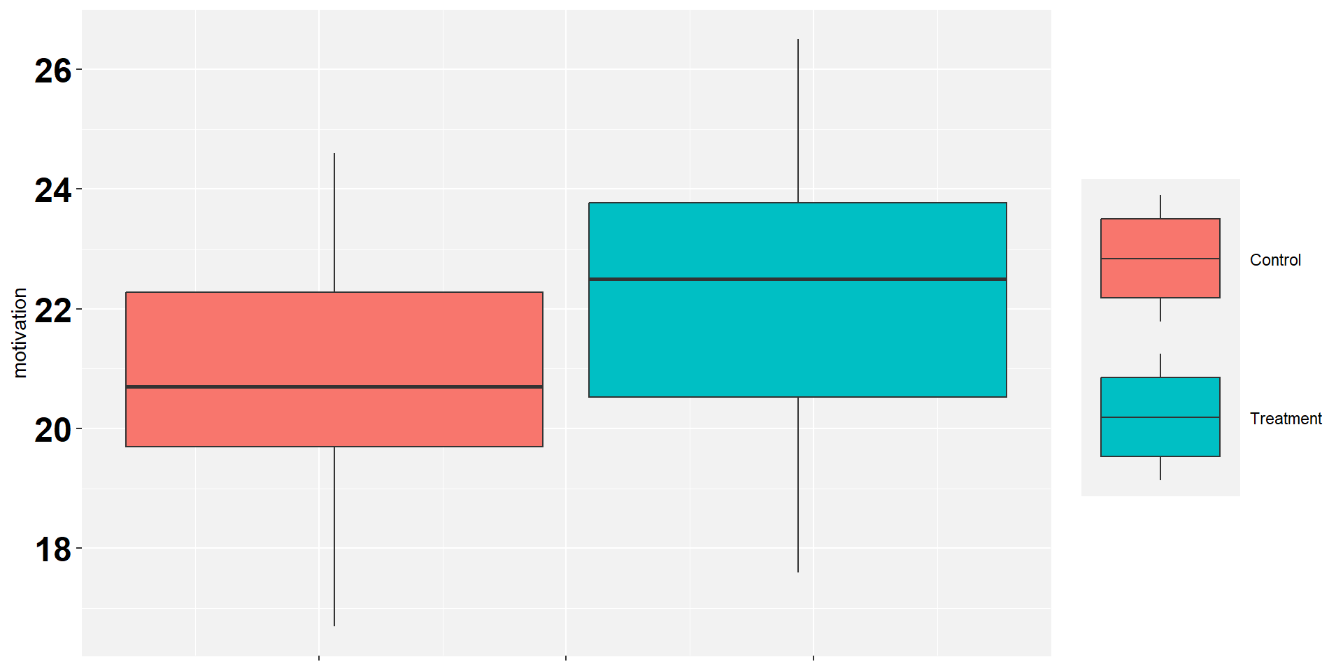
ggplot(data, aes(y=motivation, fill=group)) +   
  geom_boxplot()+
  theme(plot.title = element_text(color="black", size=30, face="bold"),
        panel.background = element_rect(fill = "grey95", colour = "grey95"),
        axis.text.y = element_text(face="bold", color="black", size = 18),
        axis.text.x = element_blank(),
        legend.title = element_blank(),
        legend.key.size = unit(3, "cm"))

Python
import pandas as pd
import seaborn as sns
import matplotlib.pyplot as plt

# Read data from Excel file
data = pd.read_excel("files/part_3_data.xlsx")

# Create a box plot of control vs treatment groups using seaborn
plt.figure(figsize=(7, 5))
sns.set(style='whitegrid')
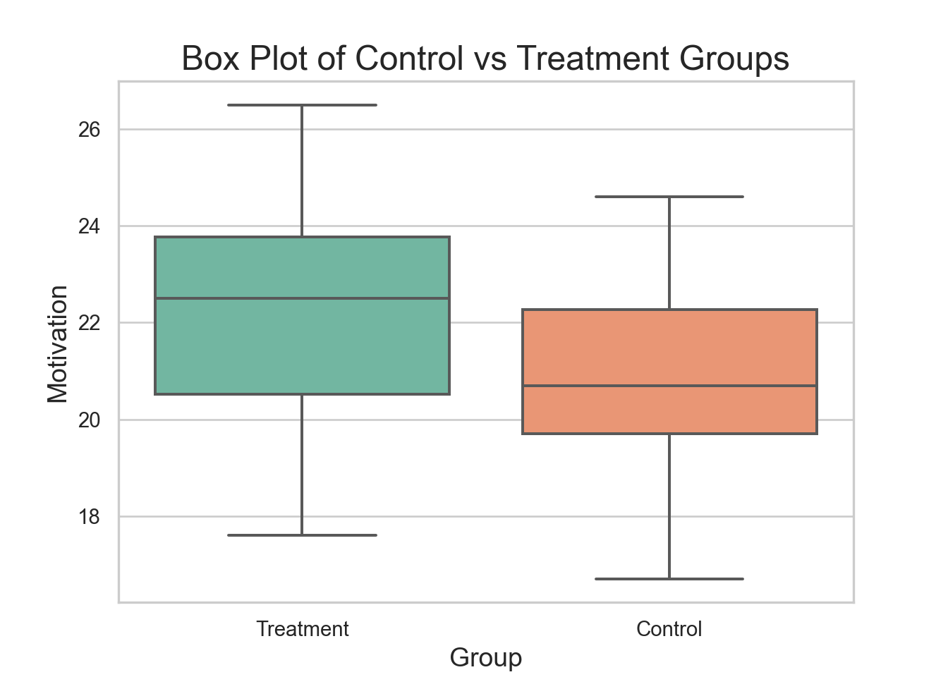
sns.boxplot(x='group', y='motivation', data=data, palette='Set2')
plt.title("Box Plot of Control vs Treatment Groups", fontsize=18)
plt.xlabel("Group", fontsize=14)
plt.ylabel("Motivation", fontsize=14)
plt.show()

Stata
import excel "files/part_3_data.xlsx", cellrange(A1:C101) firstrow clear
graph box motivation , over(group) box(1, color(black))     ytitle("Motivation")  

quietly graph export "files/graph3_5.svg", replace
(3 vars, 100 obs)

Randomization

The calculated means are below. And they are statistically different.

R
data  <- read_excel("files/part_3_data.xlsx", range = "A1:C101")
tapply(data$motivation, data$group, summary)
$Control
   Min. 1st Qu.  Median    Mean 3rd Qu.    Max. 
  16.70   19.70   20.70   20.80   22.27   24.60 

$Treatment
   Min. 1st Qu.  Median    Mean 3rd Qu.    Max. 
  17.60   20.52   22.50   22.27   23.77   26.50 
R
t.test(motivation ~ group, data = data)

    Welch Two Sample t-test

data:  motivation by group
t = -3.7301, df = 94.879, p-value = 0.0003258
alternative hypothesis: true difference in means between group Control and group Treatment is not equal to 0
95 percent confidence interval:
 -2.2493176 -0.6866824
sample estimates:
  mean in group Control mean in group Treatment 
                 20.800                  22.268 
Python
data = pd.read_excel("files/part_3_data.xlsx")
group_summary = data.groupby('group')['motivation'].describe()
print(group_summary)
           count    mean       std   min     25%   50%     75%   max
group                                                               
Control     50.0  20.800  1.780392  16.7  19.700  20.7  22.275  24.6
Treatment   50.0  22.268  2.138800  17.6  20.525  22.5  23.775  26.5
Stata
import excel "files/part_3_data.xlsx", cellrange(A1:C101) firstrow clear
bys group  : sum motivation
estpost ttest motivation , by(group)
(3 vars, 100 obs)


-------------------------------------------------------------------------------
-> group = Control

    Variable |        Obs        Mean    Std. dev.       Min        Max
-------------+---------------------------------------------------------
  motivation |         50        20.8    1.780392       16.7       24.6

-------------------------------------------------------------------------------
-> group = Treatment

    Variable |        Obs        Mean    Std. dev.       Min        Max
-------------+---------------------------------------------------------
  motivation |         50      22.268      2.1388       17.6       26.5

             |      e(b)   e(count)      e(se)       e(t)    e(df_t) 
-------------+-------------------------------------------------------
  motivation |    -1.468        100   .3935546  -3.730105         98 

             |    e(p_l)       e(p)     e(p_u)     e(N_1)    e(mu_1) 
-------------+-------------------------------------------------------
  motivation |  .0001604   .0003208   .9998396         50       20.8 

             |    e(N_2)    e(mu_2) 
-------------+----------------------
  motivation |        50     22.268 

Randomization

Is there evidence that the program has increased motivation?

  • well, if you randomly split a group of 100 people into two groups of 50, you certainly wouldn’t get the same mean motivation in both groups even if you treated them exactly alike.

  • Maybe the difference that we see is just such a difference?

How can we test this hypothesis?

Randomization

Solution:

  • Suppose the treatment had no effect, and the employees developed their motivation independently of the treatment.

  • What is the chance that the 50 employees randomly assigned to the treatment group would have an average at least 1.47 (22.27 - 20.80) points higher than the average motivation of the employees randomly assigned to the control group?

Randomization

Steps

  1. Randomly split the 100 employees that we observed in this experiment into two groups of 50.

  2. Note the difference in the mean motivation between the two groups.

  3. Repeat 1 and 2 a total of 10,000 times.

  4. Note the proportion of times the difference is at least 1.47 (22.27 - 20.80).

Randomization

R
# Load necessary libraries
data <- read_excel("files/part_3_data.xlsx", range = "A1:C101")
comb <- 10000
df <- data.frame(matrix(ncol = 2, nrow = comb))
colnames(df) <- c("order" ,"diff")
# Create the loop for randomization:
for (i in seq(from = 1, to = comb)) {
  set.seed(i)                               
  data$temp <- runif(100, min = 0, max = 1)  # Creating 100 random numbers 0 to 1
  data <- data[order(data$temp),]            # Sorting data by the random numbers generated in the previous row
  data$rank <- rank(data$temp)               # Ranking by the random numbers
# The row below defines the treatment group based on the random numbers generated. This is where we guarantee randomization
data$status_rank <- case_when(data$rank <= 50 ~ "Control_rand", data$rank > 50 ~ "Treated_rand")
# Calculate the new means of the new groups. Need to transpose data.
means <- t(as.data.frame(tapply(data$motivation, data$status_rank, mean)))
# Moving the new means to df. Each row is the difference of means
df[i, 1] <- i
df[i, 2] <- means[1, 2] - means[1, 1]
rm(means) # Deleting value
data = subset(data, select = -c(temp, rank, status_rank)) # Deleting variables
}
# Calculate a suitable binwidth for the histogram
binwidth <- (max(df$diff) - min(df$diff)) / sqrt(length(df$diff))
# Create a histogram of the differences with the calculated binwidth
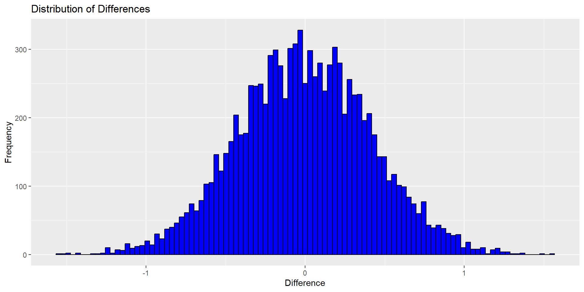
ggplot(df, aes(x = diff)) +
  geom_histogram(binwidth = binwidth, fill = "blue", color = "black") +
  labs(title = "Distribution of Differences", x = "Difference", y = "Frequency")

Stata
import excel "files/part_3_data.xlsx", cellrange(A1:C101) firstrow clear
set seed 472195         
sort group       
set obs 10000                
egen fin_order = seq() 
sort fin_order               
summarize                   
gen av_diff=.

local i = 1
while `i'<=10000 {

    sort fin_order
    gen rand_num`i' = uniform() if !missing(motivation)
    egen ordering`i' = rank(rand_num`i')
    sort ordering`i'

    gen group`i' = ""
    replace group`i' = "T" if ordering <= 50
    replace group`i' = "C" if ordering > 50 & ordering<=100
    
    qui summ motivation if group`i'=="T"
    scalar avT = `r(mean)'
    qui summ motivation if group`i'=="C"
    scalar avC = `r(mean)'
    
    sort fin_order
    replace av_diff = avT-avC in `i'
    
    drop rand_num`i' ordering`i' group`i'
    local i = `i' + 1
}
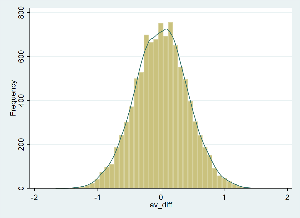
histogram av_diff, frequency kdensity  
graph export "files/graph3_6.png" , replace

Randomization

The mean difference was as far from 0 as 1.5 for only a few out of the 10,000 random divisions of the data into two groups of 50.

  • Thus, the difference between the mean motivation would almost always be less than the observed difference of 1.47 (22.27 - 20.80) if the treatment had no effect.

  • It seems reasonable to believe that the treatment caused the difference in motivation.

Measurement Error problem

Measurement Error problem

The measurement error problem has a similar statistical structure to the omitted variable bias (OVB).

  • “Classical” random measurement error for the \(y\) will inflate standard errors but will not lead to biased coefficients.

    • \(y^{*} = y + \sigma_{1}\)
    • If you estimante \(y^{*} = f(x)\), you have \(y + \sigma_{1} = x + \epsilon\)
    • \(y = x + u\)
      • where \(u = \epsilon - \sigma_{1}\)

Measurement Error problem

  • “Classical” random measurement error in x’s will bias coefficient estimates toward zero.

  • \(x^*=x+\sigma_2\)

  • Imagine that \(x^*\) is a bunch of noise. It would not explain anything. Thus, your results are biased toward zero.

Measurement Error problem

A example using one of the Wooldridge’s datasets.

R
library(foreign) 
library(jtools)
data <- read.dta("files/CEOSAL1.dta")
set.seed(2)
data$salary_noise <- data$salary + runif(length((data$salary)), min=-100, max= 100)
data$roe_noise <- data$roe + runif(length((data$roe)), min=-100, max= 100)
# OLS model 
model1 <- lm(data$salary ~ data$roe)
model2 <- lm(data$salary ~ data$roe_noise)
model3 <- lm(data$salary_noise ~ data$roe)
#summary(model1)
#summary(model2)
#summary(model3)
export_summs(model1, model2, model3, digits = 3 , model.names = c("Roe", "Roe (X) with noise", "Salary (y) with noise") )
Roe Roe (X) with noise Salary (y) with noise
(Intercept) 963.191 *** 1269.739 *** 964.058 ***
(213.240)    (97.356)    (214.588)   
data$roe 18.501              18.318    
(11.123)             (11.194)   
data$roe_noise          0.868             
         (1.593)            
N 209         209         209        
R2 0.013     0.001     0.013    
*** p < 0.001; ** p < 0.01; * p < 0.05.
Python
import pandas as pd
import numpy as np
import statsmodels.api as sm
import statsmodels.formula.api as smf
from statsmodels.iolib.summary2 import summary_col

data = pd.read_stata("files/CEOSAL1.dta")
np.random.seed(2)
# Add noise to the 'salary' and 'roe' columns
data['salary_noise'] = data['salary'] + np.random.uniform(-100, 100, len(data))
data['roe_noise'] = data['roe'] + np.random.uniform(-100, 100, len(data))
# OLS model
model1 = smf.ols(formula='salary ~ roe', data=data).fit()
model2 = smf.ols(formula='salary ~ roe_noise', data=data).fit()
model3 = smf.ols(formula='salary_noise ~ roe', data=data).fit()
# Create a summary table for all regressions
results = summary_col([model1, model2, model3], 
                      model_names=['Reg 1', 'Reg 2', 'Reg 3'],
                      stars=True,
                      float_format='%0.2f')
# Print the summary table
print(results)

=============================================
                 Reg 1     Reg 2      Reg 3  
---------------------------------------------
Intercept      963.19*** 1262.12*** 966.97***
               (213.24)  (98.19)    (213.37) 
R-squared      0.01      0.00       0.01     
R-squared Adj. 0.01      -0.00      0.01     
roe            18.50*               17.92    
               (11.12)              (11.13)  
roe_noise                1.25                
                         (1.63)              
=============================================
Standard errors in parentheses.
* p<.1, ** p<.05, ***p<.01
Stata
use "files/CEOSAL1.dta", clear
set seed 2
gen salary_noise = salary + runiform() * 200 - 100
gen roe_noise = roe + runiform() * 200 - 100
eststo: qui reg salary roe
eststo: qui reg salary roe_noise
eststo: qui reg salary_noise roe
esttab
(est1 stored)

(est2 stored)

(est3 stored)


------------------------------------------------------------
                      (1)             (2)             (3)   
                   salary          salary    salary_noise   
------------------------------------------------------------
roe                 18.50                           18.14   
                   (1.66)                          (1.63)   

roe_noise                          0.0336                   
                                   (0.02)                   

_cons               963.2***       1280.4***        966.1***
                   (4.52)         (12.71)          (4.53)   
------------------------------------------------------------
N                     209             209             209   
------------------------------------------------------------
t statistics in parentheses
* p<0.05, ** p<0.01, *** p<0.001

THANK YOU!

QUESTIONS?