Empirical Methods in Finance

Part 2

Henrique C. Martins

The challenge

Correlation & Causality

It is very common these days to hear someone say “correlation does not mean causality.”

In essence, that is true.

The killer struck during daylight. Had the sun not been out that day, the victim would have been safe.

There is a correlation, but it is clear there is no causation.

Correlation & Causality

Sometimes, there is causality even when we do not observe correlation.

The sailor is adjusting the rudder on a windy day to align the boat with the wind, but the boat is not changing direction. (Source: The Mixtape)

Note

In this example, the sailor is endogenously adjusting the course to balance the unobserved wind.

The challenge

I will discuss some issues in using plain OLS models in Finance Research (mainly with panel data).

I will avoid the word “endogeneity” as much as I can

I will also avoid the word “identification” because identification does not guarantee causality and vice-versa (Kahn and Whited 2017)

The discussion is based on Atanasov and Black (2016)

The challenge

Imagine that you want to investigate the effect of Governance on Q
- You may have more covariates explaining Q (omitted from slides)

\(𝑸_{i} = α + 𝜷_{i} × Gov + Controls + error\)

All the issues in the next slides will make it not possible to infer that changing Gov will CAUSE a change in Q

That is, cannot infer causality

1) Reverse causation

One source of bias is: reverse causation

Perhaps it is Q that causes Gov
OLS based methods do not tell the difference between these two betas:

\(𝑄_{i} = α + 𝜷_{i} × Gov + Controls + error\)

\(Gov_{i} = α + 𝜷_{i} × Q + Controls + error\)

If one Beta is significant, the other will most likely be significant too
You need a sound theory!

2) Omitted variable bias (OVB)

The second source of bias is: OVB

Imagine that you do not include an important “true” predictor of Q
Let’s say, long is: \(𝑸_{i} = 𝜶_{long} + 𝜷_{long}* gov_{i} + δ * omitted + error\)
But you estimate short: \(𝑸_{i} = 𝜶_{short} + 𝜷_{short}* gov_{i} + error\)
\(𝜷_{short}\) will be:
- \(𝜷_{short} = 𝜷_{long}\) + bias
- \(𝜷_{short} = 𝜷_{long}\) + relationship between omitted (omitted) and included (Gov) * effect of omitted in long (δ)
  - Where: relationship between omitted (omitted) and included (Gov) is: \(Omitted = 𝜶 + ϕ *gov_{i} + u\)
Thus, OVB is: \(𝜷_{short} – 𝜷_{long} = ϕ * δ\)

3) Specification error

The third source of bias is: Specification error

Even if we could perfectly measure gov and all relevant covariates, we would not know for sure the functional form through which each influences q
- Functional form: linear? Quadratic? Log-log? Semi-log?
Misspecification of x’s is similar to OVB

4) Signaling

The fourth source of bias is: Signaling

Perhaps, some individuals are signaling the existence of an X without truly having it:
- For instance: firms signaling they have good governance without having it
This is similar to the OVB because you cannot observe the full story

5) Simultaneity

The fifth source of bias is: Simultaneity

Perhaps gov and some other variable x are determined simultaneously
Perhaps there is bidirectional causation, with q causing gov and gov also causing q
In both cases, OLS regression will provide a biased estimate of the effect
Also, the sign might be wrong

6) Heterogeneous effects

The sixth source of bias is: Heterogeneous effects

Maybe the causal effect of gov on q depends on observed and unobserved firm characteristics:
- Let’s assume that firms seek to maximize q
- Different firms have different optimal gov
- Firms know their optimal gov
- If we observed all factors that affect q, each firm would be at its own optimum and OLS regression would give a non-significant coefficient
In such case, we may find a positive or negative relationship.
Neither is the true causal relationship

7) Construct validity

The seventh source of bias is: Construct validity

Some constructs (e.g. Corporate governance) are complex, and sometimes have conflicting mechanisms
We usually don’t know for sure what “good” governance is, for instance
It is common that we use imperfect proxies
They may poorly fit the underlying concept

8) Measurement error

The eighth source of bias is: Measurement error

“Classical” random measurement error for the outcome will inflate standard errors but will not lead to biased coefficients.
- \(y^{*} = y + \sigma_{1}\)
- If you estimante \(y^{*} = f(x)\), you have \(y + \sigma_{1} = x + \epsilon\)
- \(y = x + u\)
  - where \(u = \epsilon + \sigma_{1}\)
“Classical” random measurement error in x’s will bias coefficient estimates toward zero
- \(x^{*} = x + \sigma_{2}\)
- Imagine that \(x^{*}\) is a bunch of noise
- It would not explain anything
- Thus, your results are biased toward zero

9) Observation bias

The ninth source of bias is: Observation bias

This is analogous to the Hawthorne effect, in which observed subjects behave differently because they are observed
Firms which change gov may behave differently because their managers or employees think the change in gov matters, when in fact it has no direct effect

10) Interdependent effects

The tenth source of bias is: Interdependent effects

Imagine that a governance reform that will not affect share prices for a single firm might be effective if several firms adopt
Conversely, a reform that improves efficiency for a single firm might not improve profitability if adopted widely because the gains will be competed away
“One swallow doesn’t make a summer”

11) Selection bias

The eleventh source of bias is: Selection bias

If you run a regression with two types of companies
- High gov (let’s say they are the treated group)
- Low gov (let’s say they are the control group)
Without any matching method, these companies are likely not comparable
Thus, the estimated beta will contain selection bias
The bias can be either be positive or negative
It is similar to OVB

12) Self-Selection

The twelfth source of bias is: Self-Selection

Self-selection is a type of selection bias
Usually, firms decide which level of governance they adopt
There are reasons why firms adopt high governance
- If observable, you need to control for
- If unobservable, you have a problem
It is like they “self-select” into the treatment.
- Units decide whether they receive the treatment or not
Your coefficients will be biased.

13) Collider Bias (endog. selection bias)

Let’s assume an arbitrary population.

Two variables describe the population: IQ and luck.
These variables are random and normally distributed.
Let’s say that after you reach a certain level of IQ and Luck, you become successful (i.e., upper-right quadrant).
Because you are interested in successful people, you only investigate such subsample.

13) Collider Bias (endog. selection bias)

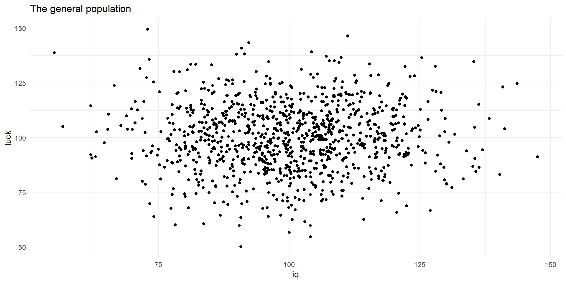
A representation of the population

R
Python
Stata

library(data.table)
library(ggplot2)
set.seed(100)
luck <- rnorm(1000, 100, 15)
iq   <- rnorm(1000, 100, 15)
pop <- data.frame(luck, iq)

ggplot(pop, aes(x = iq, y = luck)) + 
      geom_point() +
      labs(title = "The general population")  + 
  theme_minimal()

Python

import pandas as pd
import numpy as np
import matplotlib.pyplot as plt
import seaborn as sns

np.random.seed(100)

luck = np.random.normal(100, 15, 1000)
iq = np.random.normal(100, 15, 1000)
pop = pd.DataFrame({'luck': luck, 'iq': iq})

sns.set(style="whitegrid")  
plt.figure(figsize=(8, 6))
plt.scatter(pop['iq'], pop['luck'])
plt.title("The general population")
plt.xlabel("IQ")
plt.ylabel("Luck")
plt.show()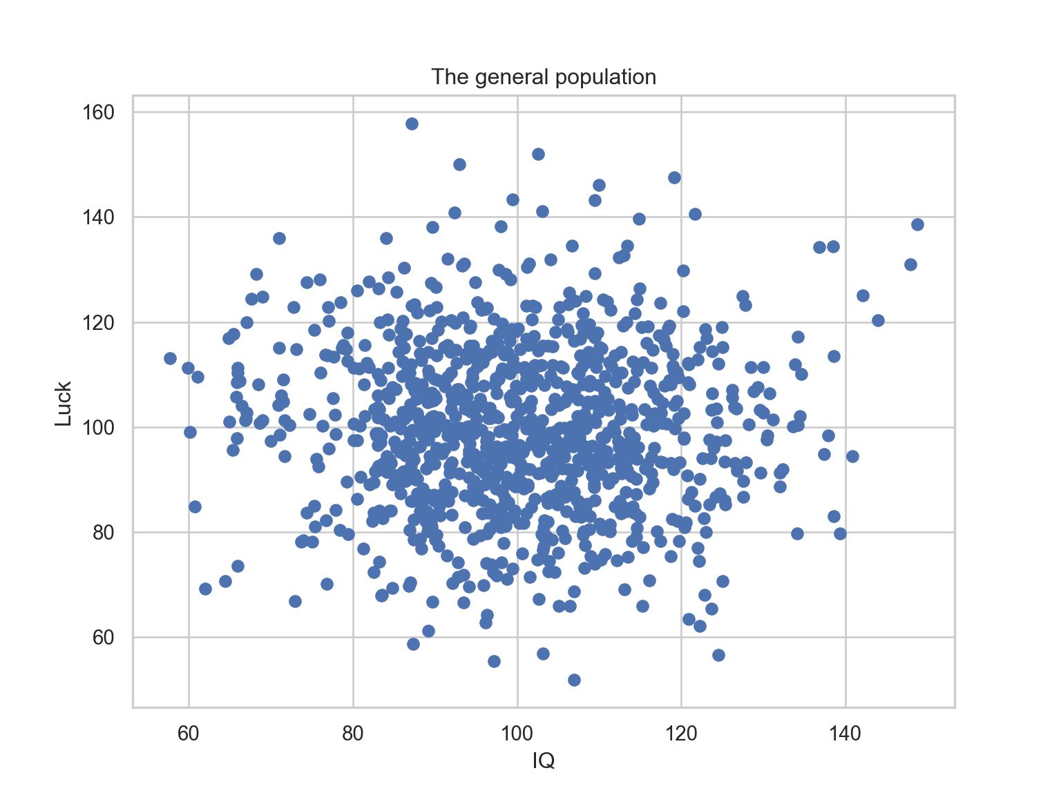

Stata

set seed 100
set obs 1000
gen luck = rnormal(100, 15)
gen iq = rnormal(100, 15)
twoway (scatter luck iq), title("The general population") 
quietly graph export figs/collider1.svg, replace

Number of observations (_N) was 0, now 1,000.

13) Collider Bias (endog. selection bias)

Important

Analyzing only successful people will suggest a negative correlation between luck and IQ.

“Success” is a collider in this example. It “collides” with luck and IQ.

R
Python
Stata

library(data.table)
library(ggplot2)
set.seed(100)
luck <- rnorm(1000, 100, 15)
iq   <- rnorm(1000, 100, 15)
pop <- data.frame(luck, iq)

pop$comb <- pop$luck + pop$iq 
successfull <- pop[pop$comb > 240, ] 

ggplot() + 
  geom_point(data = pop, aes(x = iq, y = luck)) +  
  geom_point(data = successfull, aes(x = iq, y = luck), color = "red") +  
  labs(title = "The general population & successful subpopulation") + 
  theme_minimal()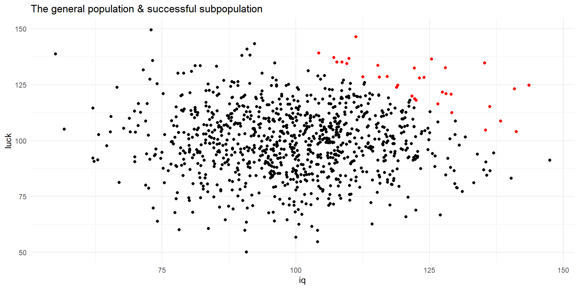

Python

import pandas as pd
import numpy as np
import matplotlib.pyplot as plt
import seaborn as sns

np.random.seed(100)

luck = np.random.normal(100, 15, 1000)
iq = np.random.normal(100, 15, 1000)
pop = pd.DataFrame({'luck': luck, 'iq': iq})

pop['comb'] = pop['luck'] + pop['iq']

successful = pop[pop['comb'] > 240]

sns.set(style="whitegrid")  # Minimalistic theme similar to theme_minimal in ggplot2
plt.figure(figsize=(8, 6))
plt.scatter(pop['iq'], pop['luck'], label="General Population", alpha=0.5)
plt.scatter(successful['iq'], successful['luck'], color='red', label="Successful Subpopulation", alpha=0.7)
plt.title("The general population & successful subpopulation")
plt.xlabel("IQ")
plt.ylabel("Luck")
plt.legend()
plt.show()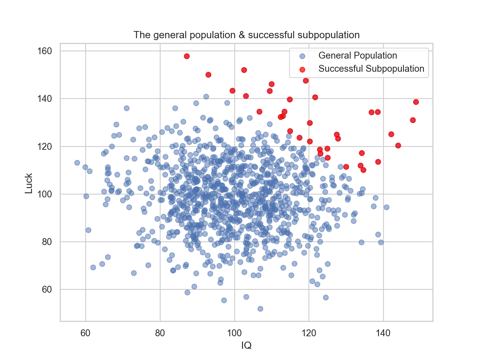

Stata

set seed 100
set obs 1000
gen luck = rnormal(100, 15)
gen iq = rnormal(100, 15)
gen comb = luck + iq
gen successful = comb > 240
twoway (scatter luck iq if successful == 0)  (scatter luck iq if successful == 1, mcolor(red)) , title("The general population & successful subpopulation") 

quietly graph export figs/collider2.svg, replace

Number of observations (_N) was 0, now 1,000.

Conclusão

Pesquisa quantitativa tem a parte quanti (métodos, modelos, etc.)…

… Mas talvez a parte mais importante seja o desenho da pesquisa (design empírico)!

Preocupações recentes em pesquisa

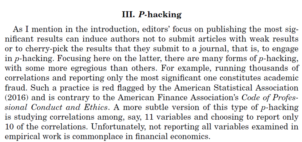
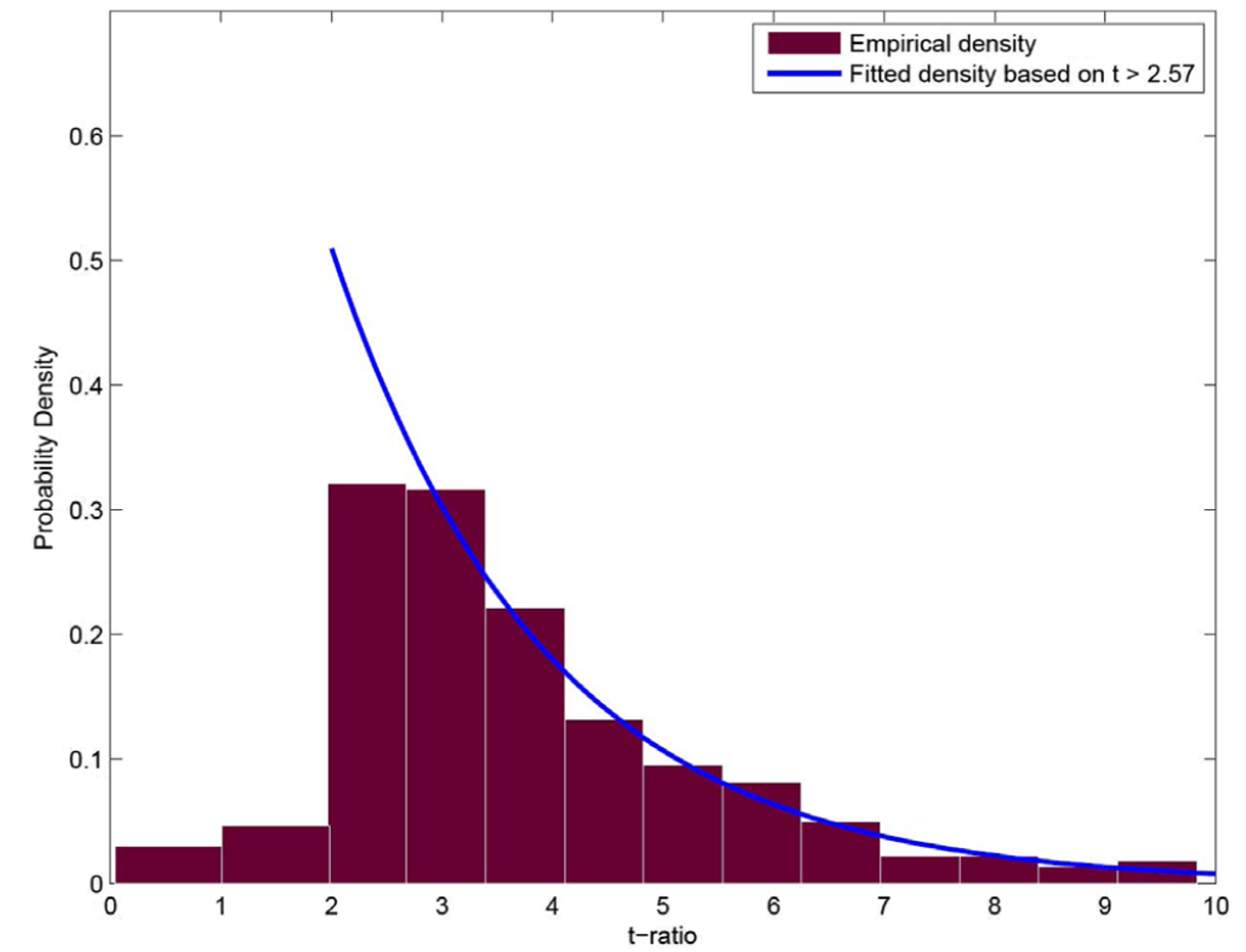
P-Hacking

Artigo original aqui.

Preocupações recentes em pesquisa

Publication bias

Artigo original aqui.

Preocupações recentes em pesquisa

Crise de replicação

Artigo original aqui.

Some fun stuff

THANK YOU!

QUESTIONS?

Henrique C. Martins