Empirical Methods in Finance

Part 11

Henrique C. Martins

Introduction

Introduction

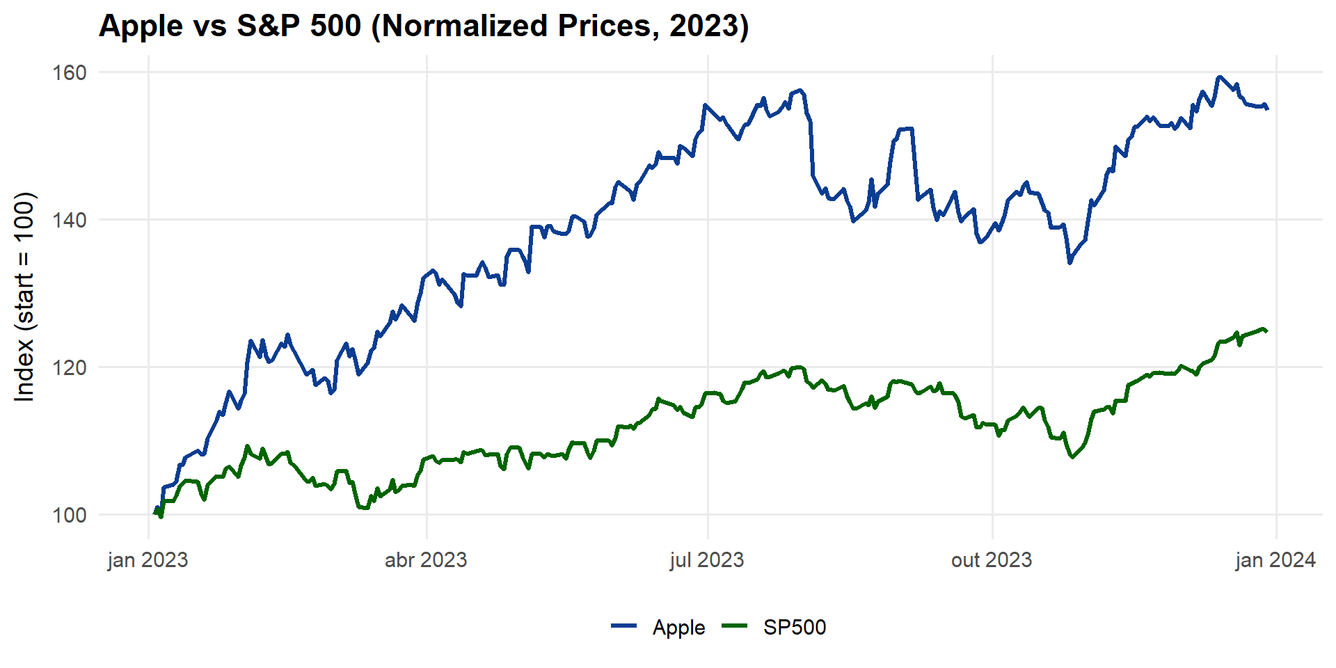
  • Event studies measure the impact of a specific event on stock returns.
  • Widely used in empirical finance:
    • Earnings announcements
    • Mergers and acquisitions
    • SEOs/IPOs
    • Credit rating downgrades
    • Regulatory changes

“Using financial market data, an event study measures the impact of a specific event on the value of a firm.” (MacKinlay, 1997)

Introduction

The event study is probably the oldest and simplest causal inference research design.

It predates experiments. It predates statistics. It probably predates human language. It might predate humans.

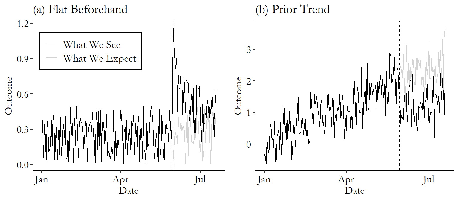
The idea is this: at a certain time, an event occured, leading a treatment to be put into place at that time. Whatever changed from before the event to after is the effect of that treatment.

(The Effect)

Introduction (The Effect)

The process for doing one of these event studies is as follows:

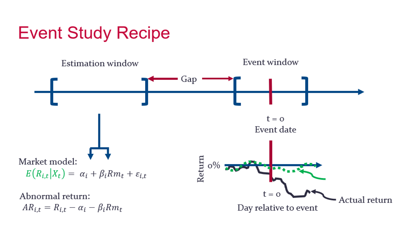
  1. Pick an “estimation period” a fair bit before the event, and an “observation period” from just before the event to the period of interest after the event.
  1. Use the data from the estimation period to estimate a model that can make a prediction of the stock’s return in each period. A popular way of doing this are:
  • Risk-adjusted returns model. Use the data from the estimation period to fit a regression describing how related the return is to other market portfolios, like the market return: \(R=\alpha + \beta \times R_m\). Then, in the observation period, use that model and the actual to predict in each period.

Introduction (The Effect)

  1. In the observation period, subtract the prediction from the actual return to get the “abnormal return.”
  • \(AR = R - \hat{R}\)
  1. Look at \(AR\) in the observation period. Nonzero values before the event imply the event was anticipated, and nonzero values after the event give the effect of the event on the stock’s return.

Introduction

Methodology

Steps of an Event Study

The central idea: measure abnormal returns (AR).

\[AR_{it} = R_{it} - E[R_{it}|X_t]\]

  1. Define event date (day 0).
  2. Select event window (e.g., [-1,+1], [-5,+5]).
  3. Select estimation window (e.g., -120 to -20 days).
  4. Estimate expected returns (Market Model, CAPM, Fama-French).
  5. Compute abnormal returns (AR).
  6. Compute cumulative abnormal returns (CAR).
  7. Test statistical significance.

Expected Return Models

  • Market Model:
    \[R_{it} = \alpha_i + \beta_i R_{mt} + \epsilon_{it}\]

  • CAPM: includes risk-free rate.

  • Fama-French: adds size (SMB), value (HML), momentum (MOM).

Choice of model depends on context, data availability, and assumptions.

Visualizing an Event

  • Day 0 = Event date
  • Look at pre- and post-event stock returns
  • Identify abnormal spikes relative to “normal” variation

Example: Earnings Announcement

Objective: Does Apple’s quarterly earnings announcement affect its stock price?

  • Event: 15 July 2023
  • Estimation window: 120 days before event
  • Event window: [-5,+5]

Example in R

Apple closing price (Adjusted)

Code
library(quantmod)
library(tidyverse)

# Data
getSymbols("AAPL", from = "2023-01-01", to = "2023-12-31", auto.assign = TRUE)
[1] "AAPL"
Code
# Ajustado (considera splits/dividendos). Se preferir o close "bruto", troque Ad(AAPL) por Cl(AAPL).
aapl_xts <- Ad(AAPL)
aapl_df  <- tibble(
  date = as.Date(index(aapl_xts)),
  adj_close = as.numeric(aapl_xts)
)

# Plot clean em azul-escuro
ggplot(aapl_df, aes(x = date, y = adj_close)) +
  geom_line(linewidth = 1.1, color = "#0b3d91") +
  labs(title = "Apple – Adjusted Closing Price (2023)",
       x = NULL, y = "USD") +
  theme_minimal(base_size = 14) +
  theme(
    panel.grid.minor = element_blank(),
    plot.title = element_text(face = "bold"),
    axis.title.y = element_text(margin = margin(r = 8))
  )

S&P 500 closing price (Adjusted)

Code
library(quantmod)
library(tidyverse)

# Data
getSymbols("^GSPC", from = "2023-01-01", to = "2023-12-31", auto.assign = TRUE)
[1] "GSPC"
Code
sp500_xts <- Ad(GSPC)
sp500_df  <- tibble(
  date = as.Date(index(sp500_xts)),
  adj_close = as.numeric(sp500_xts)
)

# Plot clean em verde-escuro
ggplot(sp500_df, aes(x = date, y = adj_close)) +
  geom_line(linewidth = 1.1, color = "#006400") +
  labs(title = "S&P 500 – Adjusted Closing Price (2023)",
       x = NULL, y = "Index Points") +
  theme_minimal(base_size = 14) +
  theme(
    panel.grid.minor = element_blank(),
    plot.title = element_text(face = "bold"),
    axis.title.y = element_text(margin = margin(r = 8))
  )

Apple vs S&P 500 (Normalized to 100)

Code
library(quantmod)
library(tidyverse)

# Data
getSymbols("AAPL", from = "2023-01-01", to = "2023-12-31", auto.assign = TRUE)
[1] "AAPL"
Code
getSymbols("^GSPC", from = "2023-01-01", to = "2023-12-31", auto.assign = TRUE)
[1] "GSPC"
Code
# Preços ajustados
aapl_xts  <- Ad(AAPL)
sp500_xts <- Ad(GSPC)

# Normalizar para 100 no início
aapl_norm  <- as.numeric(aapl_xts)  / as.numeric(first(aapl_xts))  * 100
sp500_norm <- as.numeric(sp500_xts) / as.numeric(first(sp500_xts)) * 100

df <- tibble(
  date = as.Date(index(aapl_xts)),
  Apple = aapl_norm,
  SP500 = sp500_norm
) %>% pivot_longer(-date, names_to = "Asset", values_to = "Index")

# Plot
ggplot(df, aes(x = date, y = Index, color = Asset)) +
  geom_line(linewidth = 1.1) +
  scale_color_manual(values = c("Apple" = "#0b3d91", "SP500" = "#006400")) +
  labs(title = "Apple vs S&P 500 (Normalized Prices, 2023)",
       x = NULL, y = "Index (start = 100)", color = NULL) +
  theme_minimal(base_size = 14) +
  theme(
    panel.grid.minor = element_blank(),
    plot.title = element_text(face = "bold"),
    legend.position = "bottom",
    axis.title.y = element_text(margin = margin(r = 8))
  )

Step 1 – Compute Returns and Market Model

We now move from prices to daily returns.
This allows us to estimate the Market Model using OLS on the estimation window.

Code
library(quantmod)
library(tidyverse)

# Compute daily returns
ret_aapl <- dailyReturn(Ad(AAPL))
ret_mkt  <- dailyReturn(Ad(GSPC))

# Define event date and estimation window (120 days before)
event_date <- as.Date("2023-07-15")
estimation_window <- index(ret_aapl) < event_date & 
                     index(ret_aapl) >= (event_date - 180)  # ~6 months before

# Estimate Market Model via OLS
fit <- lm(ret_aapl[estimation_window] ~ ret_mkt[estimation_window])

summary(fit)

Call:
lm(formula = ret_aapl[estimation_window] ~ ret_mkt[estimation_window])

Residuals:
      Min        1Q    Median        3Q       Max 
-0.018873 -0.005409 -0.000416  0.004732  0.033962 

Coefficients:
                            Estimate Std. Error t value Pr(>|t|)    
(Intercept)                0.0018071  0.0007359   2.456   0.0155 *  
ret_mkt[estimation_window] 1.0980088  0.0831552  13.204   <2e-16 ***
---
Signif. codes:  0 '***' 0.001 '**' 0.01 '*' 0.05 '.' 0.1 ' ' 1

Residual standard error: 0.008142 on 122 degrees of freedom
Multiple R-squared:  0.5883,    Adjusted R-squared:  0.585 
F-statistic: 174.4 on 1 and 122 DF,  p-value: < 2.2e-16

Step 2 – Compute Abnormal Returns (AR)

Once we have the estimated parameters (\(\hat{\alpha}\), \(\hat{\beta}\)),we can compute expected returns and the abnormal returns:

\(\hat{R}_{i,t} = \hat{\alpha} + \hat{\beta} R_{m,t}\)

\(AR_{i,t} = R_{i,t} - \hat{R}_{i,t}\)

Code
# Predicted returns from the Market Model
pred <- predict(fit, newdata = data.frame(ret_mkt = ret_mkt))

# Abnormal returns
ar <- ret_aapl - pred

head(ar, 10)   # first 10 abnormal returns
           daily.returns
2023-01-03  0.0004223688
2023-01-04  0.0255949386
2023-01-05 -0.0040247814
2023-01-06  0.0142143417
2023-01-09 -0.0107640774
2023-01-10  0.0034305933
2023-01-11  0.0195048773
2023-01-12 -0.0144933794
2023-01-13  0.0055727897
2023-01-17  0.0211888536

AR > 0: Apple outperformed the market on that day

AR < 0: Apple underperformed the market on that day

Step 3 – Compute CAR

To capture the aggregate effect of the event, we sum abnormal returns over the event window:

\(CAR_{i}(t_1,t_2) = \sum_{t=t_1}^{t_2} AR_{i,t}\)

Code
# Define event window: 5 days before and after
window <- (index(ret_aapl) >= (event_date - 5)) &
          (index(ret_aapl) <= (event_date + 5))

# Cumulative abnormal returns
car <- cumsum(ar[window])

car
           daily.returns
2023-07-10  -0.025708796
2023-07-11  -0.029544737
2023-07-12  -0.022166677
2023-07-13  -0.032003133
2023-07-14  -0.035762294
2023-07-17  -0.006024236
2023-07-18  -0.025249174
2023-07-19  -0.031461287
2023-07-20  -0.059505828

A positive CAR suggests good news (value creation).

A negative CAR suggests bad news (value destruction).

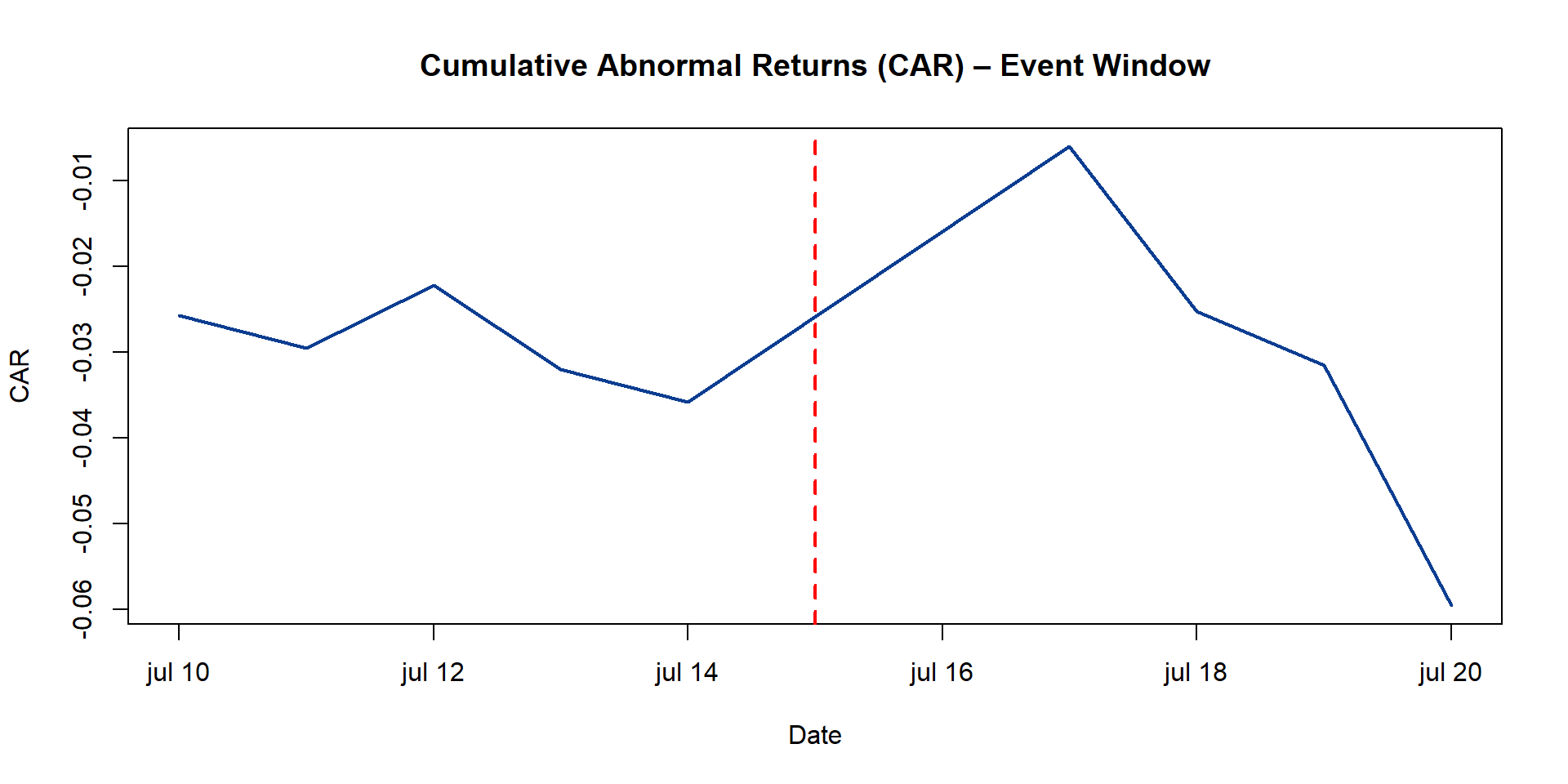
Step 4 – Visualize CAR

Code
# Extract abnormal returns only for the event window
ar_window <- ar[window]

# Recalculate CAR starting at 0
car <- cumsum(as.numeric(ar_window))

# Plot corrected CAR
plot(index(ar_window), car, type = "l", col = "#0b3d91", lwd = 2,
     main = "Cumulative Abnormal Returns (CAR) – Event Window",
     xlab = "Date", ylab = "CAR")
abline(v = event_date, col = "red", lwd = 2, lty = 2)

What is the CAR in this window?

  • Estimation window: 120 trading days before the event (used to estimate the market model).
  • Event window: [-5, +5] days around the event date (used to measure the abnormal impact).
  • The CAR (Cumulative Abnormal Return) is the sum of abnormal returns across this event window.
Code
ar_window <- ar[window]                  # abnormal returns in the event window [-5,+5]
car <- cumsum(as.numeric(ar_window))     # cumulative abnormal returns, starting at 0
CAR_total <- last(car)                   # CAR over the full event window
CAR_total
[1] -0.05950583

Robustness table

CAR robustness across estimation and event windows
est_window_days event_window n_est n_event alpha_hat beta_hat CAR t_CAR
60 [-10,+10] 41 15 0.00073 0.862 -0.0260 -0.95
60 [-3,+3] 41 5 0.00073 0.862 0.0039 0.22
60 [-5,+5] 41 9 0.00073 0.862 -0.0198 -0.81
120 [-10,+10] 82 15 0.00077 1.102 -0.0327 -1.14
120 [-3,+3] 82 5 0.00077 1.102 -0.0025 -0.13
120 [-5,+5] 82 9 0.00077 1.102 -0.0276 -1.10
180 [-10,+10] 124 15 0.00181 1.098 -0.0481 -1.68
180 [-3,+3] 124 5 0.00181 1.098 -0.0076 -0.40
180 [-5,+5] 124 9 0.00181 1.098 -0.0367 -1.47

Extensions

Extensions and Practical Challenges

  • Multiple events
    • Often researchers examine a wave of events (e.g., several M&As in one industry, multiple SEOs).
    • Challenge: heterogeneity across firms and event timing. Aggregation must be justified.

Extensions and Practical Challenges

  • Clustering of events
    • Many events occur on the same date (e.g., quarterly earnings announcements).
    • Standard errors may be underestimated if cross-sectional dependence is ignored.
    • Solutions: event-time portfolios, clustered or robust standard errors.

Extensions and Practical Challenges

  • Confounding events
    • Other major news may coincide with the focal event (e.g., macro policy change).
    • Makes it difficult to attribute abnormal returns exclusively to the event of interest.

Extensions and Practical Challenges

  • Long-horizon event studies
    • Extending the event window to months/years raises econometric issues.
    • CARs accumulate model error and are sensitive to the choice of expected-return model.
    • Interpretation becomes less about short-term information effects, more about long-run performance.

Final Comments

Final Comments

  • Event studies are powerful and widely used.
  • Results depend heavily on:
    • Correct identification of the event
    • Appropriate choice of estimation model
    • Robustness checks

Easy to run, hard to interpret.

🙋‍♂️ Any Questions?

Thank You!

Henrique C. Martins