Empirical Methods in Finance

Part 10

Henrique C. Martins

Introduction IV

Imagine the following model

\[Ln(wage)=\alpha + \beta_1 educ + \epsilon\]

We can infer that educ is correlated with ability, but the latter is in the error term.

educ in this case is “endogenous”.

\[Cov(educ, \epsilon) \neq 0\]

Introduction IV

The setup of an IV is

Suppose that we have an observable variable z that satisfies these two assumptions:

z is uncorrelated with u:

\[Cov(z, \epsilon) = 0\]

z is correlated with x:

\[Cov(z, x) \neq 0\]

Then, we call z an instrumental variable for x, or sometimes simply an instrument for x.

Introduction IV

Before we continue,

IV is not a model, it is an estimation method

I’ll call it a Design.

Do not say, I estimated an IV model (more often than it should be).

Instrumental Variables

Imagine that you have one independent variable that is “endogenous”:

\(Cov(x_k,\mu)\neq 0\)
You may have many other independent variables not “endogenous”

In this situation:

\(B_k\) is biased
The other betas will likely be biased as well, since it is unlikely that all other Xs are not correlated with \(x_k\)

Instrumental Variables

\(x_k\) is the endogenous variable.

It has “good” variation:
- the part that varies that is not correlated with \(\mu\)
It has “bad” variation:
- the part that varies that is correlated with \(\mu\)

Let’s assume now that you can find an instrument \(z\)

The instrument \(z\) is correlated with \(X_k\), but only the “good” variation, not the “bad”.
The instrument \(z\) does not explain \(y\) directly, only through \(x_k\).
- Only through condition.

Instrumental Variables

Relevance Condition

The instrument \(z\) is correlated with \(x_k\).

This assumption is easy to test. Simply run a regression of \(x=f(z, all\; Xs)\) and check the significance of the \(\beta_z\).
This is called the first stage of an IV regression
- Tip: Always show the beta coefficient and the R2 (even if low) of the first-stage.

Exclusion Condition

The instrument \(z\) is not correlated with \(\mu\).

That is \(cov(z,\mu) = 0\)
As all correlations with \(\mu\), you cannot test this prediction. You have to rely on the theory, create a story about that.

Instrumental Variables

An example of IV Murray.

Instrumental Variables

An example of IV Murray.

Instrumental Variables

Mixtape

Good instruments should feel weird

Parents with two same-gender kids are more likely to try a third kid than a diverse-gender pair of parents.

So, you may use the gender of the kids as instrument for the likelihood of the mother go back to the labor market.

Angrist’s example

Remember the Fuzzy RDD.

There is the treatment
There is the position (before or after the cut)

The position is an indication of receiving or not the treatment, but it is not definitive.

Thus, we can use the position as an IV for the treatment.

Angrist’s example

Mixtape

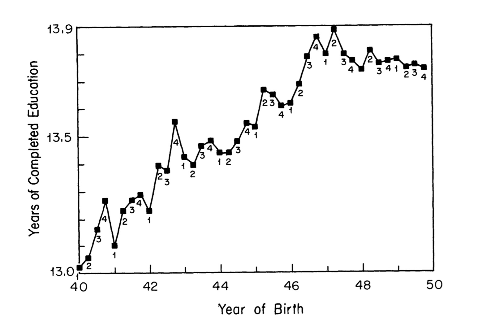
One of the more seminal papers in instrumental variables for the modern period is Angrist and Krueger (1991).

Their idea is simple and clever; a quirk in the United States educational system is that a child enters a grade on the basis of his or her birthday.

For a long time, that cutoff was late December. If children were born on or before December 31, then they were assigned to the first grade. But if their birthday was on or after January 1, they were assigned to kindergarten.

Thus two people—one born on December 31 and one born on January 1—were exogenously assigned different grades.

Everyone is forced to leave school when 16.

Angrist’s example

Mixtape

Angrist and Krueger had the insight that that small quirk was exogenously assigning more schooling to people born later in the year.

The person born in December would reach age 16 with more education than the person born in January

Angrist’s example

Mixtape

What is the instrument here?

Angrist’s example

Mixtape

What is the instrument here?

The instrument is the quarter of birth.

People born in the 3rd and 4th quarter receive more education than others due to compulsory schooling.

Two-stage least squares (2SLS)

One of the more intuitive instrumental variables estimators is the 2SLS.

The first stage is

\[x_k = \delta + \delta_1 z + \delta_2 x_1 + . . .+ \delta_n x_n + \mu\]

Then, you predict \(x_k\) using the first stage.

“predict” means that you are finding the “response” Y of the equation after estimating the coefficients

\[\hat{x_k} = \hat{\delta} + \hat{\delta_1} z + \hat{\delta_2} x_1 + . . . + \hat{\delta_n} x_n \]

Then, the second stage is:

\[y = \alpha + \beta_1 \hat{x_k} + \beta_2 x_1 + . . .+ \beta_n x_n + \mu\]

The idea using \(\hat{x_k}\) is that it represents only the variation that is not correlated with \(\mu\).

Instrumental Variables

We can write that:

\[\beta_1= \frac{Cov(z,y)}{Cov(z,x_k)}\]

It shows that \(\beta_1\) is the population covariance between z and y divided by the population covariance between z and x.
Notice how this fails if z and x are uncorrelated, that is, if \(Cov(z, x) = 0\)

\[\beta_1= \frac{\sum_{i=1}^n(z_i-\bar{z})(y_i-\bar{y})}{\sum_{i=1}^n(z_i-\bar{z})(x_i-\bar{x})}\]

Notice that if \(z\) and \(x\) are the same (i.e., perfect correlation), \(\beta_1\) above is the OLS \(\beta\)

\[\beta_1= \frac{\sum_{i=1}^n(x_i-\bar{x})(y_i-\bar{y})}{\sum_{i=1}^n(x_i-\bar{x})^2}\]

Weak Instruments

I did not demonstrate here, but we can say that (see pp; 517-18 Wooldridge):

though IV is consistent when \(z\) and \(u\) are uncorrelated and \(z\) and \(x\) have any positive or negative correlation, IV estimates can have large standard errors, especially if \(z\) and \(x\) are only weakly correlated.

This gives rise to the week instruments problem.

We can write the probability limit of the IV estimator:

\[plim \hat{\beta_{iv}} = \beta_1 + \frac{Corr(z,\mu)}{Corr(z,x)} \times \frac{\sigma_{\mu}}{\sigma_x}\]

It shows that, even if \(Corr(z,\mu)\) is small, the inconsistency in the IV estimator can be very large if \(Corr(z,x)\) is also small.

Weak Instruments

Two tips:

Look at the F-stat of the first-stage. It should not be low.
The sign of the coefficient in the first stage should be as expected.
Look at the S.E. When the instrument is week, the S.E., are even larger than it should be.

One more tip,

Avoid computing the first stage by hand, it would give wrong estimates of the S.E. in the second stage.

Example

OLS

Stata

Stata

use files/mroz.dta , clear
reg lwage educ

      Source |       SS           df       MS      Number of obs   =       428
-------------+----------------------------------   F(1, 426)       =     56.93
       Model |  26.3264237         1  26.3264237   Prob > F        =    0.0000
    Residual |  197.001028       426  .462443727   R-squared       =    0.1179
-------------+----------------------------------   Adj R-squared   =    0.1158
       Total |  223.327451       427  .523015108   Root MSE        =    .68003

------------------------------------------------------------------------------
       lwage | Coefficient  Std. err.      t    P>|t|     [95% conf. interval]
-------------+----------------------------------------------------------------
        educ |   .1086487   .0143998     7.55   0.000     .0803451    .1369523
       _cons |  -.1851969   .1852259    -1.00   0.318    -.5492674    .1788735
------------------------------------------------------------------------------

Example

The IV estimate of the return to education is 5.9%, which is barely more than one-half of the OLS estimate. This suggests that the OLS estimate is too high and is consistent with omitted ability bias.

Stata

Stata

use files/mroz.dta , clear
ivreg lwage (educ =fatheduc ) , first

First-stage regressions
-----------------------

      Source |       SS           df       MS      Number of obs   =       428
-------------+----------------------------------   F(1, 426)       =     88.84
       Model |  384.841983         1  384.841983   Prob > F        =    0.0000
    Residual |  1845.35428       426  4.33181756   R-squared       =    0.1726
-------------+----------------------------------   Adj R-squared   =    0.1706
       Total |  2230.19626       427  5.22294206   Root MSE        =    2.0813

------------------------------------------------------------------------------
        educ | Coefficient  Std. err.      t    P>|t|     [95% conf. interval]
-------------+----------------------------------------------------------------
    fatheduc |   .2694416   .0285863     9.43   0.000     .2132538    .3256295
       _cons |   10.23705   .2759363    37.10   0.000     9.694685    10.77942
------------------------------------------------------------------------------


Instrumental variables 2SLS regression

      Source |       SS           df       MS      Number of obs   =       428
-------------+----------------------------------   F(1, 426)       =      2.84
       Model |  20.8673618         1  20.8673618   Prob > F        =    0.0929
    Residual |  202.460089       426  .475258426   R-squared       =    0.0934
-------------+----------------------------------   Adj R-squared   =    0.0913
       Total |  223.327451       427  .523015108   Root MSE        =    .68939

------------------------------------------------------------------------------
       lwage | Coefficient  Std. err.      t    P>|t|     [95% conf. interval]
-------------+----------------------------------------------------------------
        educ |   .0591735   .0351418     1.68   0.093    -.0098994    .1282463
       _cons |   .4411035   .4461018     0.99   0.323    -.4357311    1.317938
------------------------------------------------------------------------------
Instrumented: educ
 Instruments: fatheduc

Final Comments

When you have only one Z, you can say that the model is just identified.

But you can have multiple IVs, in which case you will say that the model is overidentified.

You can implement IV design just as before
The relevance and exclusion assumptions are there as well.

Assuming that both conditions are satisfied, you will have more asymptotic efficiency in the IV estimates.

Final Comments

It is rare to have multiple Zs. You should be happy if you have a good one!

But if you do have multiple IVs, you can test their quality…

If they are all valid, you should get consistent estimates…
… even if you use only a subset of them.
So the test is about how similar the estimates are if you use subsets of IVs.

But this test does not give really an answer about whether the IVs are good.

This always come from theory.

Final Comments

Some more comments:

If you have an interaction term between \(x_1\) and \(x_2\), and \(z\) is the instrument for \(x_1\), you can “create” the instrument \(zx_2\) for \(x_2\).

GMM uses lagged variables as instruments. But, this is not a good decision if the variables are highly serially correlated.

Lagged total assets is not a good instrument for total assets.

Using the average-group of variable X is also problematic (i.e., the industry average own. concentration as IV of firm-level own. concentration)

This is no different than a group FE, making hard to believe in the exclusion restriction.

THANK YOU!

QUESTIONS?

Henrique C. Martins