Empirical Methods in Finance
Part 1


Você nunca sabe o resultado do caminho que não toma.
Como fazemos na prática?
Exemplo de modelo empírico:
\(Y_{i} = α + 𝜷_{1} × X_i + Controls + error\)
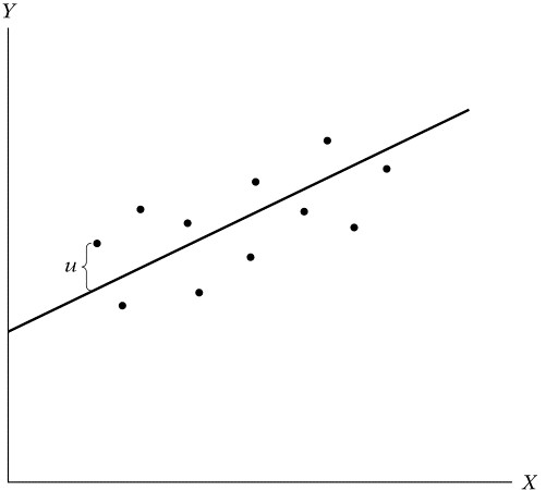
Uma vez que estimemos esse modelo, temos o valor, o sinal e a significância do \(𝜷\).
Se o Beta for significativamente diferente de zero e positivo –> X e Y estão positivamente correlacionados.
O problema? Os pacotes estatísticos que utilizamos sempre “cospem” um beta. Seja ele com ou sem viés.
Cabe ao pesquisador ter um design empírico que garanta que o beta estimado tenha validade interna.
Como fazemos na prática?
A decisão final é baseada na significância do Beta estimado. Se significativo, as variáveis são relacionadas e fazemos inferências em cima disso.
Contudo, sem um design empírico inteligente, o beta encontrado pode ter literalmente qualquer sinal e significância.
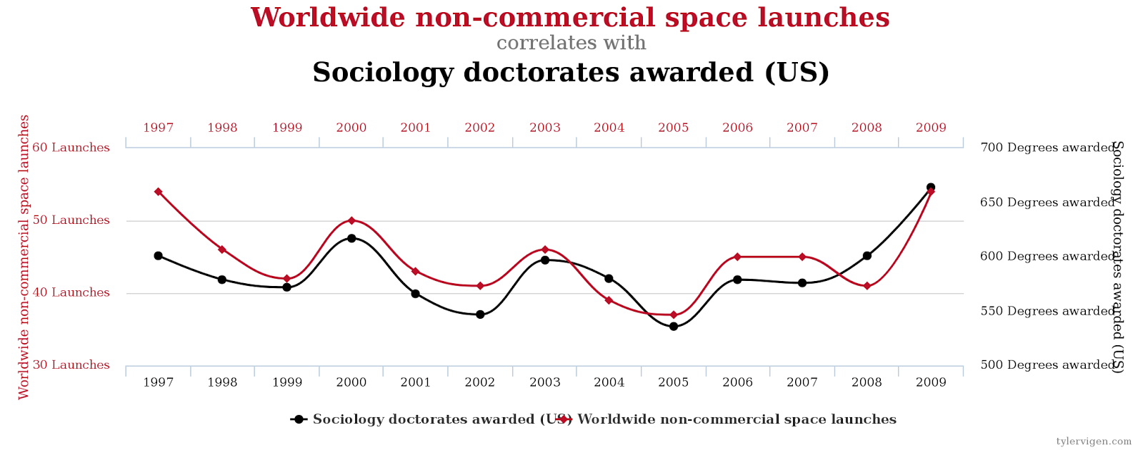
Exemplo desses problemas
Veja esse site.
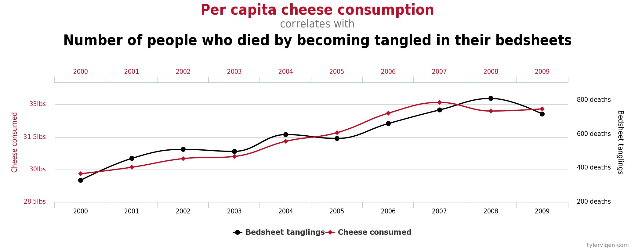
Exemplo desses problemas
Veja esse site.
Selection bias - We see I
R
library(data.table)
library(ggplot2)
# Generate Data
n = 10000
set.seed(100)
x <- rnorm(n)
y <- rnorm(n)
data1 <- 1/(1+exp( 2 - x  -  y))
group  <- rbinom(n, 1, data1)

# Data Together
data_we_see     <- subset(data.table(x, y, group), group==1)
data_all        <- data.table(x, y, group)

# Graphs
ggplot(data_we_see, aes(x = x, y = y)) +
      geom_point(aes(colour = factor(-group)), size = 1) +
      geom_smooth(method=lm, se=FALSE, fullrange=FALSE)+
      labs( y = "", x="", title = "The observations we see")+
      xlim(-3,4)+ ylim(-3,4)+
      theme(plot.title = element_text(color="black", size=30, face="bold"),
            panel.background = element_rect(fill = "grey95", colour = "grey95"),
            axis.text.y = element_text(face="bold", color="black", size = 18),
            axis.text.x = element_text(face="bold", color="black", size = 18),
            legend.position = "none")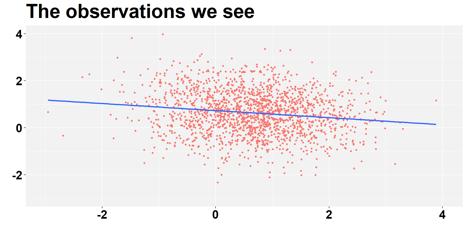
Python
import numpy as np
import pandas as pd
import matplotlib.pyplot as plt
import seaborn as sns

n = 10000
np.random.seed(100)
x = np.random.normal(size=n)
y = np.random.normal(size=n)
data1 = 1 / (1 + np.exp(2 - x - y))
group = np.random.binomial(1, data1, n)

data_we_see = pd.DataFrame({'x': x[group == 1], 'y': y[group == 1], 'group': group[group == 1]})
data_all = pd.DataFrame({'x': x, 'y': y, 'group': group})

sns.set(style='whitegrid')
plt.figure(figsize=(7, 5))
plt.scatter(data_we_see['x'], data_we_see['y'], c=-data_we_see['group'], cmap='viridis', s=20)
sns.regplot(x='x', y='y', data=data_we_see, scatter=False, ci=None, line_kws={'color': 'blue'})
plt.title("The observations we see", fontsize=18)
plt.xlabel("")
plt.ylabel("")
plt.show()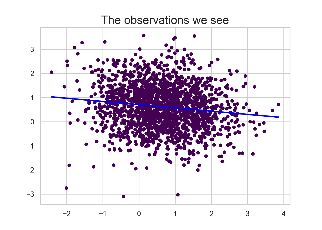
Stata
clear all
set seed 100
set obs 10000
gen x = rnormal(0,1)
gen y = rnormal(0,1)
gen data1 = 1 / (1 + exp(2 - x - y))
gen group = rbinomial(1, data1)
twoway (scatter x y if group == 1, mcolor(black) msize(small))    (lfit y x if group == 1, color(blue)),title("The observations we see", size(large) ) xtitle("") ytitle("")
quietly graph export figs/graph1.svg, replace
Selection bias - All I
R
ggplot(data_all, aes(x = x, y = y,  colour=group)) +
  geom_point(aes(colour = factor(-group)), size = 1) +
  geom_smooth(method=lm, se=FALSE, fullrange=FALSE)+
  labs( y = "", x="", title = "All observations")+
  xlim(-3,4)+ ylim(-3,4)+
  theme(plot.title = element_text(color="black", size=30, face="bold"),
      panel.background = element_rect(fill = "grey95", colour = "grey95"),
      axis.text.y = element_text(face="bold", color="black", size = 18),
      axis.text.x = element_text(face="bold", color="black", size = 18),
      legend.position = "none")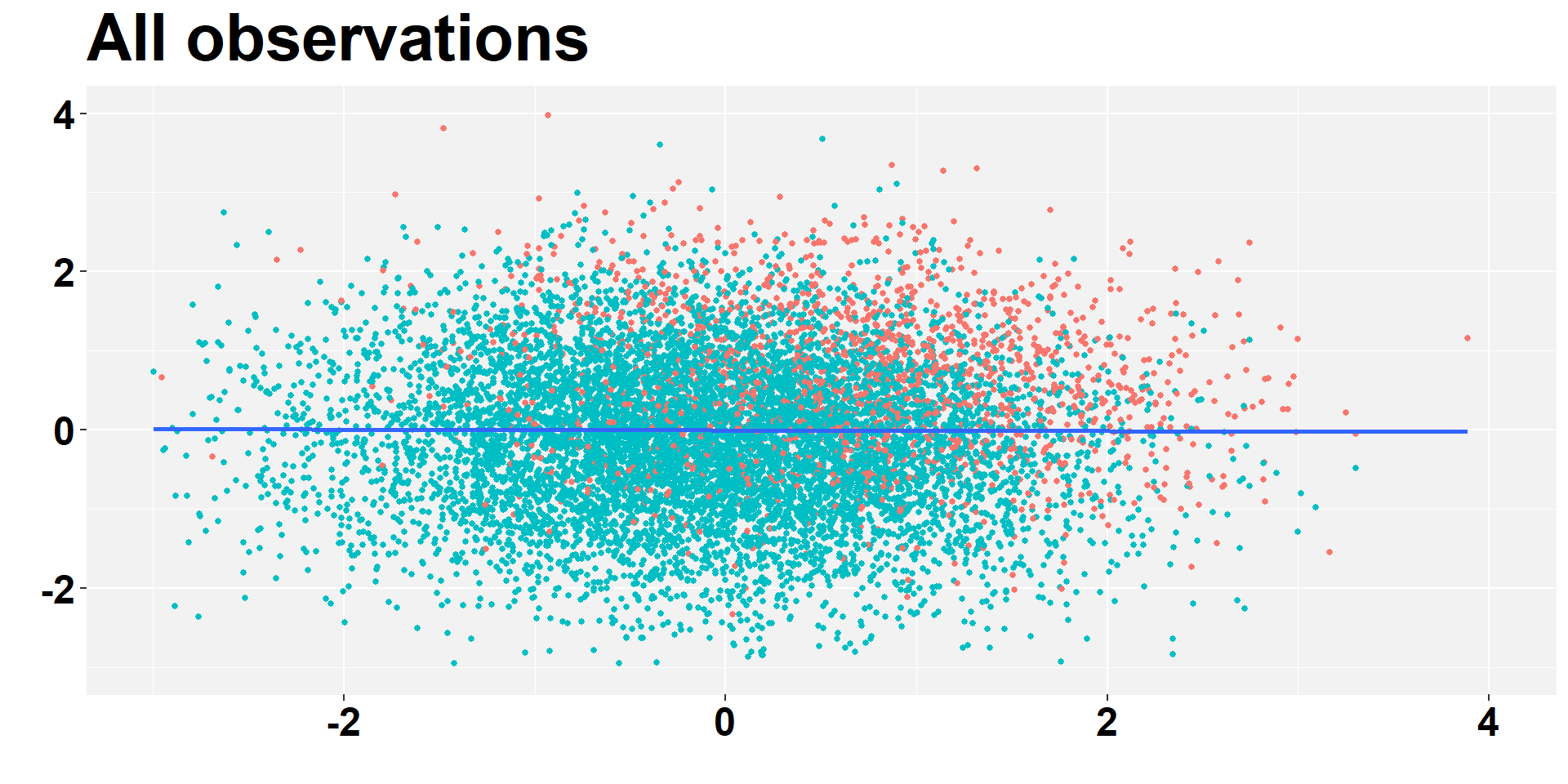
Python
import pandas as pd
import seaborn as sns
import matplotlib.pyplot as plt

sns.set(style='whitegrid')
plt.figure(figsize=(6, 4))
sns.scatterplot(data=data_all, x='x', y='y', hue='group', palette=['blue', 'red'], s=20)
sns.regplot(data=data_all, x='x', y='y', scatter=False, ci=None, line_kws={'color': 'blue'})
plt.title("All observations", fontsize=18)
plt.xlabel("")
plt.ylabel("")
plt.legend(title="Group", labels=["0", "1"], loc="upper left")

plt.gca().get_legend().remove()
plt.show()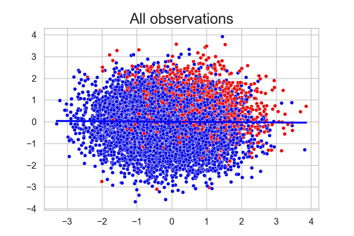
Number of observations (_N) was 0, now 10,000.
Exemplo desses problemas

Source: Angrist
Não podemos pegar dois caminhos.
Exemplo desses problemas

Source: Angrist
Não podemos comparar pessoas que não são comparáveis.
🙋♂️ Any Questions?
Thank You!