Inferência Causal em Pesquisas de Finanças: Problemas e Soluções

Enanpad 2024

Henrique C. Martins

17-09-2024

Correlation & Causality

It is very common these days to hear someone say “correlation does not mean causality.”

In essence, that is true.

The killer struck during daylight. Had the sun not been out that day, the victim would have been safe.
There is a correlation, but it is clear there is no causation.

Sometimes, there is causality even when we do not observe correlation.

The sailor is adjusting the rudder on a windy day to align the boat with the wind, but the boat is not changing direction. (Source: The Mixtape)

Note

In this example, the sailor is endogenously adjusting the course to balance the unobserved wind.

The challenge

I will discuss some issues in using plain OLS models in Finance Research (mainly with panel data).

I will avoid the word “endogeneity” as much as possible.
- This word refers to the violation of the Conditional Mean Independence (CMI) assumption, meaning that \(x\) and \(\mu\) are correlated.

I will also avoid the word “identification” because identification does not guarantee causality and vice-versa (Kahn and Whited 2017)

The discussion is mainly based on Atanasov and Black (2016)

The challenge

Imagine that you want to investigate the effect of Governance on Q
- You may have more covariates explaining Q (omitted from slides)

\(𝑸_{i} = α + 𝜷 × Gov_{i} + Controls + error\)

All the issues in the next slides will make it not possible to infer that changing Gov will CAUSE a change in Q

That is, cannot infer causality

1) Reverse causation

Perhaps it is \(Q\) that causes \(Gov\).
OLS based methods do not tell the difference between these two betas:
- \(Q_{i} = \alpha + \beta × Gov_{i} + Controls + \epsilon\)
- \(Gov_{i} = \alpha + \beta × Q_{i} + Controls + \epsilon\)
If one Beta is significant, the other will most likely be significant too.
You need a sound theory (and possibly play with lags, might not be enough)!

2) Simultaneity

Perhaps \(Gov\) and \(Q\) are determined simultaneously.
That is, there is a third variable causing both.
An OLS regression will provide a biased estimate of the effect.
Also, the sign might be wrong.

3) Omitted variable bias (OVB)

Imagine that you do not include an important “true” predictor of \(Q\)
Let’s say, long is: \(𝑸_{i} = \alpha_{long} + \beta_{long}* Gov_{i} + δ * omitted + error\)
But you estimate short: \(𝑸_{i} = \alpha_{short} + \beta_{short}* Gov_{i} + error\)
\(\beta_{short}\) will be:
- \(\beta_{short} = \beta_{long}\) + bias
- \(\beta_{short} = \beta_{long}\) + relationship between omitted (omitted) and included (Gov) * effect of omitted in long (δ)
  - Where: relationship between omitted (omitted) and included (Gov) is: \(Omitted = \alpha + ϕ *Gov_{i} + \mu\)
Thus, OVB is: \(\beta_{short} – \beta_{long} = ϕ * δ\)

4) Bad Controls

Bad controls are variables that are also outcome of the treatment (i.e., \(Gov\)) being studied.
A Bad control could very well be a dependent variable of \(Gov\) as well.
Good controls are variables that you can think as being fixed at the time of the treatment.
- \(𝑄_{i} = \alpha + \beta × Gov_{i} + Controls + \epsilon\)
Assuming you also have something that is the consequence of good governance (e.g., Novo Mercado dummy). Should you include it in the model?
No. In this case, the coefficient of interest no longer has a causal interpretation.

Warning

It is not hard to come up with stories of why a control is a bad control.

5) Collider bias

Collider bias occurs when an independent variable and outcome each influence a third variable and that variable or collider is included in the regression.

In a way, a collider is a bad control.
While a bad control makes you underestimate the effect, a collider creates spurious correlation between the X and the Y.

In the analysis below

\(Q_{i} = \alpha + \beta × Gov_{i} + Controls + \epsilon\)

Including, for instance, CEO Reputation (assuming that both \(Q\) and \(Gov\) influences CEO Reputation) creates a false correlation between \(Gov\) and \(Q\).

You may estimate a significant association even when there is none.

6) Specification error

\(Q_{i} = \alpha + \beta × Gov_{i} + Controls + \epsilon\)

Even if we could perfectly measure \(Gov\) and all relevant covariates, we would not know for sure the functional form through which each influences \(Q\).
- Functional form: linear? Quadratic? Log-log? Semi-log?
Misspecification of x’s is similar to OVB.

7) Signaling

Perhaps, some individuals are signaling the existence of an X without truly having it:
- For instance: firms signaling they have good governance without it
This is similar to the OVB because you cannot observe the full story.

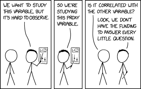
8) Construct validity

Some constructs (e.g. \(Gov\)) are complex and sometimes have conflicting mechanisms.
We usually don’t know for sure what “good” governance is, for instance.
It is common to use imperfect proxies, that may poorly fit the underlying concept.

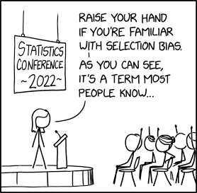
9) Measurement error

“Classical” random measurement error in x’s will bias the coefficient toward zero
- \(x^{*} = x + \sigma_{2}\)
- Imagine that \(x^{*}\) is a bunch of noise. It would not explain anything.
- Thus, your results are biased toward zero.
“Classical” random measurement error in the Y will inflate standard errors but will not lead to biased coefficients.
- \(y^{*} = y + \sigma_{1}\)
- If you estimante \(y^{*} = f(x)\), you have \(y + \sigma_{1} = x + \epsilon\)
- \(y = x + u\)
  - where \(u = \epsilon + \sigma_{1}\)

10) Heterogeneous effects

Maybe the causal effect of \(Gov\) on \(Q\) depends on observed and unobserved firm characteristics:
- Let’s assume that firms seek to maximize \(Q\).
- Different firms have different optimal \(Gov\).
- Firms know their optimal \(Gov\).
- If we observed all factors that affect \(Q\), each firm would be at its own optimum and OLS regression would give a non-significant coefficient.
In such case, we may find a positive or negative relationship.
Neither is the true causal relationship.

11) Observation bias

This is analogous to the Hawthorne effect, in which observed subjects behave differently because they are observed.
Firms which change gov may behave differently because their managers or employees think the change in \(Gov\) matters, when in fact it has no direct effect.

12) Selection bias

If you run a regression with two types of companies
- High gov (let’s say they are the treated group)
- Low gov (let’s say they are the control group)
Without any matching method, these companies are likely not comparable
- Apples compared to oranges
Thus, the estimated beta will contain selection bias, which can be either be positive or negative

13) Self-Selection

Self-selection is a type of selection bias. Usually, firms decide which level of governance they adopt
It is like they “self-select” into the treatment.
- Units decide whether they receive the treatment or not
There are reasons why firms adopt high governance
- If observable, you need to control for. If unobservable, you have a problem.

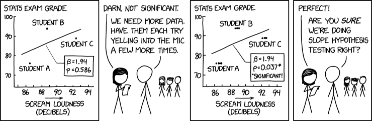
Important

More data is not necessarily a solution, you need a sound empirical design.

THANK YOU!

QUESTIONS?

Henrique C. Martins